Calculating the Mean and Median of a Data Set: Background You’ll Need 4

Comparing Groups with Histograms

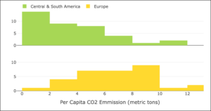
The following graph compares the distribution of per capita CO2 emissions between two groups: countries in Central and South America and countries in Europe.

Two histograms are shown. In the first histogram, it shows the per capita CO2 Emission in metric tons (x-axis) and the number of Central and South American countries that produce those amounts of emissions. 14 countries emitted between 0 and 2 metric tons. 9 countries emitted between 2 and 4 metric tons. 8 countries emitted between 4 and 6 metric tons. 4 countries emitted between 6 to 8 metric tons. 1 country emitted between 8 and 10 metric tons. 2 countries emitted between 10 and 12 metric tons. In the second histogram, it shows the per capita CO2 Emission in metric tons (x-axis) and the number of European countries that produce those amounts of emissions. 1 country emitted between 0 and 2 metric tons. 4 countries emitted between 2 and 4 metric tons. 7 countries emitted between 4 and 6 metric tons. 7 countries emitted between 6 and 8 metric tons. 9 countries emitted between 8 and 10 metric tons. 1 country emitted between 10 and 12 metric tons. 2 countries emitted 12 or more metric tons.

question 13

question 14

If you feel comfortable reading, interpreting, and comparing histograms, please move on to the next section and activity.