Drawing inferences from boxplots
Now let’s look at the data from the 2017 Tax Reform bill.
The data from the Tax Policy Center in the table below separates income groups into quintiles. Quintiles divide data sets into five parts, from the lowest [latex]20[/latex]% of values up to the highest [latex]20[/latex]% of values.
The Tax Policy Center released the following data about the actual tax cuts households experienced because of the 2017 Tax Reform bill.[1]
| Household Tax Cuts | |
| Income Group | Mean Tax Cut |
| Lowest Quintile | $[latex]40[/latex] |
| Second Quintile | $[latex]320[/latex] |
| Middle Quintile | $[latex]780[/latex] |
| Fourth Quintile | $[latex]1,480[/latex] |
| Top Quintile | $[latex]5,790[/latex] |
| Top 1 Percent | $[latex]32,650[/latex] |
| Top 0.1 Percent | $[latex]89,060[/latex] |
Compare the 2017 Tax Reform data with the hypothetical data displayed in boxplots A and B below: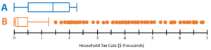
question 9
question 10
question 11
question 12
video placement
Wrap up: “There are many perspectives to take and questions to answer when trying to sort out as complicated a situation as this one. We are only presented a small amount of information in this activity so we limited ourselves to questions we could answer using the data we had. It is of interest, though, to compare these tax cuts given in dollar amounts to their equivalencies in terms of percent of peoples’ incomes. [voice over the table given in the hidden text below]. The Tax Policy Center also provides this information. The top income groups received both the largest cuts in dollar amounts but also the largest percent growth in after-tax income as a result of the bill (the top 0.1 percent don’t follow this trend, however). But hopefully you’ve been able to understand from this activity how boxplots provide a quick glance, a summary, of the data to make comparisons based on median, skew, outliers, and percentiles. Let’s take a look at a few general five-number summaries to make sure you feel good about what you’ve learned here.” — Provide a few five-number summaries and ask students to sketch boxplots of them. Then show the answers for comparison. — “You’ve seen that boxplots provide visual summaries of quantitative variables that can be used to compare the distributions of multiple populations. Hopefully, you feel that you are now comfortable using boxplots to compare and draw inferences.”
- Tax Policy Center. (2018, February 16). T18-0025 - The Tax Cuts and Jobs Act (TCJA): All provisions and individual income tax provisions; distribution of federal tax change by expanded cash income percentile, 2018. https://www.taxpolicycenter.org/model-estimates/individual-income-tax-provisions-tax-cuts-and-jobs-act-tcja-february-2018/t18-0025 ↵