Learning Objectives
- Use a probability distribution for a continuous random variable to estimate probabilities and identify unusual events.
Previously, we examined the probability distribution for foot length. For foot length and for all other continuous random variables, the probability distribution can be approximated by a smooth curve called a probability density curve.
Recall that these smooth curves are mathematical models. We use a mathematical model to describe a probability distribution so that we can use technology and the equation of this model to estimate probabilities. (As we mentioned earlier, we do not study the equation for this curve in this course, but every statistical package uses this equation, and the area under the corresponding curve, to estimate probabilities.)

As in a probability histogram, the total area under the density curve equals 1, and the curve represents probabilities by area. To find the probability that X is in an interval, find the area above the interval and below the density curve.
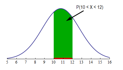
For example, if X is foot length, let’s find P(10 < X < 12), the probability that a randomly chosen male has a foot length anywhere between 10 and 12 inches. This probability is the area above the interval 10 < X < 12 and below the curve. We shaded this area with green in the following graph.
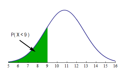
If, for example, we are interested in P(X < 9), the probability that a randomly chosen male has a foot length of less than 9 inches, we have to find the area shaded in green below:
Comments
- We have seen that for a discrete random variable like shoe size, P(X < 9) and P(X ≤ 9) have different values. In other words, including the endpoint of the interval changes the probability. In contrast, for a continuous random variable like foot length, the probability of a foot length of less than or equal to 9 will be the same as the probability of a foot length of strictly less than 9. In other words, P(X < 9) = P(X ≤ 9). Visually, in terms of our density curve, the area under the curve up to and including a certain point is the same as the area up to and excluding the point. This is because there is no area over a single point. There are infinitely many possible values for a continuous random variable, so technically the probability of any single value occurring is zero!
- It should be clear now why the total area under any probability density curve must be 1. The total area under the curve represents P (X gets a value in the interval of its possible values). Clearly, according to the rules of probability, this must be 1, or always true.
- Density curves, like probability histograms, may have any shape imaginable as long as the total area underneath the curve is 1. Each density curve is a mathematical model with an equation that is used to find the area underneath the curve.
Let’s Summarize
The probability distribution of a continuous random variable is represented by a probability density curve. The probability that X has a value in any interval of interest is the area above this interval and below the density curve.

Candela Citations
- Concepts in Statistics. Provided by: Open Learning Initiative. Located at: http://oli.cmu.edu. License: CC BY: Attribution