Example

Winter-run Chinook Salmon on the Sacramento River

The U.S. Endangered Species Act lists nine populations of Chinook salmon as either threatened or endangered. One such population is the winter-run Chinook salmon of the Sacramento River in northern California. The Chinook was first listed as endangered in 1994.

A number of factors contributed to the decline of the Chinook on the Sacramento River. Chief among these was the construction of the Red Bluff Diversion Dam in 1967. The dam deprived a large number of adult salmon access to necessary coldwater spawning grounds.

Researchers collected data on the Chinook population at the Red Bluff Dam. This data suggests that the population declined from about 40,000 in 1970 to below 200 in 1994. Click here to see the data.

Here is a scatterplot of the data for the years 1970 through 1994. The scatterplot has a nonlinear form with a negative association between the variables. In other words, we see that the population is declining.

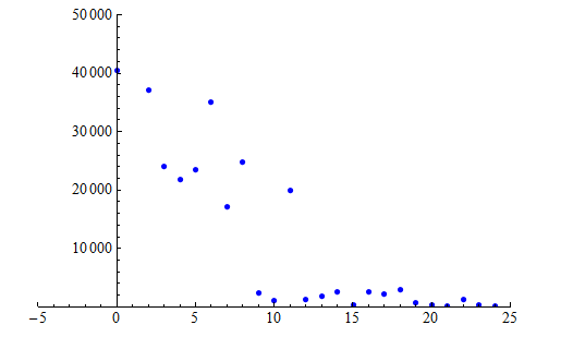
Note: We defined t, our explanatory variable, to be Number of years after 1970. The response variable is the Number of Chinook salmon present in the Sacramento River.

Our goal is to model the decline of the Sacramento River Chinook population.

In the scatterplot below, we fit an exponential model to the data for the years 1970 through 1994. Notice that this model summarizes the pattern in the data, but the relationship is not as strong as we saw in the eagle data. There is more scatter about the exponential curve.

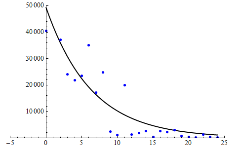
The equation of the exponential model is Predicted Chinook population = 49,304 (0.854)^t.

Now we use the exponential model to make predictions about the Chinook population. We expect fairly large prediction errors because the association is not strong.

In 1994 (t = 24), there were 186 Chinook salmon in the Sacramento River, according to the data.

According to the model: Predicted Chinook population = 49,304 (0.854)²⁴ = 1,117.

The exponential model overestimates the number of Chinook salmon by 1,117 − 186 = 931 for that year. We can tell from the graph that this prediction error is small relative to the prediction error for most of the other years. (The data point for 1994, when t = 24, is much closer to the curve than are other data points.)

In 2003 (t = 33), there were 9,757 Chinook, according to the data.

According to the model: Predicted Chinook population = 49,304 (0.854)³³ = 270.

The exponential model underestimates the number of Chinook by 9,757 − 270 = 9,487. This is a huge prediction error. But wait – this is an example of extrapolation: 2003 falls outside of the range of the data used to find the model. The model gives unreliable estimates for years outside the range of 1975 through 1994. If you look at the data table, you will see that the Chinook population started to increase again after 1994, with large increases in 2002 and 2003. Because the pattern changes after 1994, this exponential model gives unreliable predictions for years after 1994. (This turnaround was the result of the removal of two dams on the Sacramento River and opening the dam gates for 8 months a year at the Red Bluff Diversion Dam to allow for fish migration to winter spawning areas.)

Note: In Examining Relationships: Quantitative Data, we investigated techniques for assessing the fit of a linear model, such as residual plots, r² and s_e. We do not formally investigate residuals for exponential functions in this course. We also do not develop formal techniques for assessing the fit of an exponential model.