Let’s Summarize
In Inference for Two Proportions, we learned two inference procedures to draw conclusions about a difference between two population proportions (or about a treatment effect): (1) a confidence interval when our goal is to estimate the difference and (2) a hypothesis test when our goal is to test a claim about the difference. Both types of inference are based on the sampling distribution.
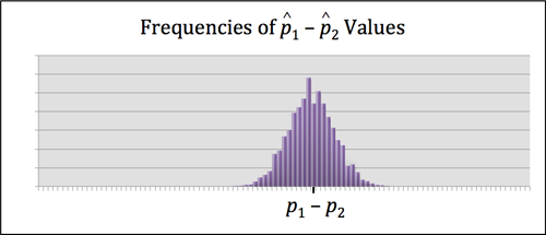
The Distribution of the Differences in Sample Proportions
In the section “Distribution of Differences in Sample Proportions,” we learned about the sampling distribution of differences between sample proportions.
We used simulation to observe the behavior of sample differences when we select random samples from two populations. Every simulation began with an assumption about the difference between the two population proportions. From the simulated sampling distribution, we could determine if a sample difference observed in the data was likely or unlikely. A data result that is unlikely to occur in the sampling distribution provides evidence that our original assumption about the difference in the population proportions is probably incorrect. This logic is similar to the logic of hypothesis testing.
Because samples vary, we do not expect sample differences to always equal the population difference. Every sample difference has some error. We used simulations to observe the amount of error we expected to see in sample differences. The “typical” amount of error in the sampling distribution connects to the margin of error in a confidence interval.
We also used simulations to describe the shape, center, and spread of the sampling distribution. Later we developed a mathematical model for the sampling distribution with formulas for the mean of the sample differences and the standard deviation of the sample differences. We call this standard deviation the standard error because it represents an estimate for the average error we see in sample differences.
The mean of sample differences between sample proportions is equal to the difference between the population proportions, p1 − p2.
The standard error of differences between sample proportions is related to the population proportions and the sample sizes.
[latex]\sqrt{\frac{{p}_{1}(1-{p}_{1})}{{n}_{1}}+\frac{{p}_{2}(1-{p}_{2})}{{n}_{2}}}[/latex]
A normal model is a good fit for the sampling distribution of differences between sample proportions under certain conditions. We use a normal model if the counts of expected successes and failures are at least 10. For those who like formulas, this translates into saying the following four calculations must all be at least 10.
- n1p1
- n1(1 − p1)
- n2p2
- n2(1 − p2)
Estimating the Difference between Two Population Proportions
In the section “Estimate the Difference between Population Proportions,” we learned how to calculate a confidence interval to estimate the difference between two population proportions (or to estimate a treatment effect).
Every confidence interval has the form:
[latex]\mathrm{statistic}\text{}±\text{}\mathrm{margin}\text{}\mathrm{of}\text{}\mathrm{error}[/latex]
To estimate a difference in population proportions (or a treatment effect), the statistic is a difference in sample proportions. So the confidence interval is
[latex](\mathrm{difference}\text{}\mathrm{in}\text{}\mathrm{sample}\text{}\mathrm{proportions})\text{}±\text{}\mathrm{margin}\text{}\mathrm{of}\text{}\mathrm{error}[/latex]
Also, since we do not know the values of the population proportions, we estimate the standard error by using sample proportions in the formula for the margin of error.
[latex]{Z}_{c}\sqrt{\frac{{\stackrel{ˆ}{p}}_{1}(1-{\stackrel{ˆ}{p}}_{1})}{{n}_{1}}+\frac{{\stackrel{ˆ}{p}}_{2}(1-{\stackrel{ˆ}{p}}_{2})}{{n}_{2}}}[/latex]
Here are the critical Z-values for commonly used confidence levels.
| Confidence Level | Critical Value Zc |
| 90% | 1.645 |
| 95% | 1.960 |
| 99% | 2.576 |
The connection between the confidence level and critical Z-value depends on the use of a normal model. We use a normal model if each sample has at least 10 successes and failures.
We practiced interpreting confidence intervals and confidence levels. For example, we say we are “95% confident” that the population difference lies within the calculated confidence interval. We do not say there is a 95% chance that the population difference lies within the calculated interval. 95% confident means that in the long run 95% of the confidence intervals will contain the population differences.
Hypothesis Test for a Difference in Two Population Proportions
In the section “Hypothesis Test for a Difference in Population Proportions,” we tested claims regarding the difference between two population proportions (or a treatment effect).
In testing such claims, the null hypothesis is
- H0: p1 − p2 = 0
The alternative hypothesis is one of three:
- Ha: p1 − p2 < 0, or
- Ha: p1 − p2 > 0, or
- Ha: p1 − p2 ≠ 0
These are equivalent to the following comparisons of p1 and p2.
- Ha: p1 < p2
- Ha: p1 > p2
- Ha: p1 ≠ p2
We use the same criteria for determining if a normal model is a good fit for the sampling distribution: each sample must have at least 10 successes and failures.
In a hypothesis test, we assume the null hypothesis is true. Since we do not have values for p1 and p2, we again use sample data to estimate them. In the null hypothesis the population proportions are equal, so we create a single-value estimate for the population proportions using the pooled proportion.
[latex]\stackrel{ˆ}{p}\text{}=\text{}\frac{{x}_{1}\text{}+\text{}{x}_{2}}{{n}_{1}\text{}+\text{}{n}_{2}}[/latex]
With this pooled proportion, we estimate the standard error to compute the Z-test statistic for the hypothesis test. We can always view the z-score as the error in the statistic divided by the standard error. In a hypothesis test, we predict the error on the basis of the null, and we estimate the standard error.
[latex]\begin{array}{l}Z\text{}=\text{}\frac{\mathrm{predicted}\text{}\mathrm{error}\text{}\mathrm{in}\text{}\mathrm{the}\text{}\mathrm{statistic}}{\mathrm{predicted}\text{}\mathrm{standard}\text{}\mathrm{error}}\\ Z\text{}=\text{}\frac{({\stackrel{ˆ}{p}}_{1}-{\stackrel{ˆ}{p}}_{2})-({p}_{1}-{p}_{2})}{\sqrt{\frac{\stackrel{¯}{p}(1-\stackrel{¯}{p})}{{n}_{1}}+\frac{\stackrel{¯}{p}(1-\stackrel{¯}{p})}{{n}_{2}}}}\end{array}[/latex]
If the conditions for approximate normality are met, this standardized statistic is approximately normal. This fact allows us to determine a P-value using computer software.
Whenever the P-value is less than or equal to the level of significance, we reject the null hypothesis in favor of the alternative. Otherwise, we fail to reject (but do not support) the null hypothesis.
Because our conclusions are based on probability, there is always a chance that our data will lead us to an incorrect conclusion. We make a type I error when we reject a true null hypothesis. We make a type II error when we fail to reject a false null hypothesis. These errors are not the result of a mistake. They are due to chance.
The level of significance, α, is the probability of a type I error. The probability of a type II error is harder to calculate. We did not learn to calculate type II error. Small values of α increase the probability of a type II error. Larger samples sizes decrease the probability of a type II error.
Finally, we should always remember “garbage in, garbage out.” If random selection or random assignment is not used to produce the data, we should not do inference.
Candela Citations
- Concepts in Statistics. Provided by: Open Learning Initiative. Located at: http://oli.cmu.edu. License: CC BY: Attribution