Learning Objectives
- Use a normal probability distribution to estimate probabilities and identify unusual events.
In Summarizing Data Graphically and Numerically, we encountered data sets, such as height and weight, with distributions that are fairly symmetric with a central peak. We call these bell-shaped.
Many variables, such as weight, shoe sizes, foot lengths, and other human physical characteristics, exhibit these properties. The symmetry indicates that the variable is just as likely to take a value a certain distance below its mean as it is to take a value that same distance above its mean. The bell shape indicates that values closer to the mean are more likely, and it becomes increasingly unlikely to take values far from the mean in either direction.
We use a mathematical model with a smooth bell-shaped curve to describe these bell-shaped data distributions. These models are called normal curves or normal distributions. They were first called “normal” because the pattern occurred in many different types of common measurements.
The general shape of the mathematical model used to generate a normal curve looks like this:

Observations of Normal Distributions
There are many normal curves. Even though all normal curves have the same bell shape, they vary in their center and spread.
Because normal curves are mathematical models, we use Greek letters to represent the mean and standard deviation of a normal curve. The mean of a normal distribution locates its center. We use the Greek letter μ (pronounced “mu” ) to represent the mean. We use the Greek letter σ (pronounced “sigma”) to represent the standard deviation of a normal distribution. The standard deviation determines the spread of the distribution. In fact, the shape of a normal curve is completely determined by specifying its standard deviation. As we will see, if two normal distributions have the same standard deviation, then the shapes of their normal curves will be identical.
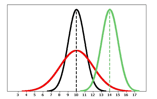
Following are some observations we can make as we look at the figure above:
- The black and the red normal curves have means or centers at μ = 10. However, the red curve is more spread out and thus has a larger standard deviation. Notice that the red normal curve is also shorter. This makes sense because these curves are probability density curves, so the area under each curve has to be 1.
- The black and the green normal curves have the same standard deviation or spread.
Comment
- We use [latex]\stackrel{¯}{x}[/latex] to represent the mean of data in a sample. We use μ to represent the mean of a density curve defined by a mathematical model.
- We use SD or [latex]{s}_{x}[/latex] to represent the standard deviation of data in sample. We use σ to represent the standard deviation of a density curve defined by a mathematical model.
The normal curve has a central role in statistical inference, as we’ll see in Linking Probability to Statistical Inference. Understanding the normal distribution is an important step in the direction of our overall goal, which is to relate sample means or proportions to population means or proportions. The goal of this section is to help you better understand normal random variables and their distributions.
All normal curves share a basic geometry. While the mean locates the center of a normal curve, it is the standard deviation that is in control of the geometry. To see how, let’s examine a few pictures of normal curves to see what they reveal.
Example
One Standard Deviation on Each Side of the Mean
Let’s start with a random variable X that has a normal distribution with mean = 10 and standard deviation = 2. Let’s practice our new notation. Here we would write μ = 10 and σ = 2 .
The normal curve for X is shown below.

As expected, the mean μ = 10 is located at the center of the normal curve. The other two arrows point to values 1 standard deviation on each side of the mean.
The point 1 standard deviation less than the mean is represented by μ − σ . Since μ = 10 and σ = 2, this point is located at 10 − 2 = 8, as shown.
The point 1 standard deviation more than the mean is represented by μ + σ . Since μ = 10 and σ = 2, this point is located at 10 + 2 = 12, as shown.
You will notice we have indicated that the area of the green region is 0.68. So we can say that the probability of X being between 8 and 12 equals 0.68.
Or, using our probability notation, we could write:
[latex]P(8 Now here is an interesting fact. If we took any normal distribution and drew a similar picture, the probability that a value falls within 1 standard deviation of the mean is always the same. Here are several ways to express this idea: This is a big deal. It is one of the things that makes normal curves special. In general, probability density curves for continuous random variables with different shapes don’t have this special property. Let’s put this idea in context. If the weight of babies at birth follows a normal distribution with mean μ = 3,500 grams and standard deviation σ = 600 grams, then we can conclude that most babies – that is, about 68% – will weigh somewhere between 2,900 grams (i.e., 3,500 − 600 = 2,900) and 4,100 grams (i.e., 3,500 + 600 = 4,100).
Candela Citations
- Concepts in Statistics. Provided by: Open Learning Initiative. Located at: http://oli.cmu.edu. License: CC BY: Attribution