Learning Objectives
- Use mean and standard deviation to describe a distribution.
Deciding Which Measurements to Use
We now have a choice between two measurements of center and spread. We can use the median with the interquartile range, or we can use the mean with the standard deviation. How do we decide which measurements to use?
Our next examples show that the shape of the distribution and the presence of outliers helps us answer this question.
Example
Homework Scores with an Outlier
Here are two summaries of the same set of homework scores earned by a student: a boxplot and an SD hatplot. Notice that the distribution of scores has an outlier. This student has mostly high homework scores with one score of 0. Here are some observations about the homework data.
- Five-number summary: low: 0 Q1: 82 Q2: 84.5 Q3: 89 high: 100
- Median is 84.5 and IQR is 7
- Mean = 81.8, SD = 17.6
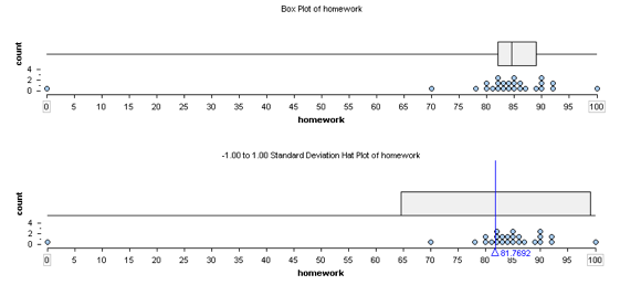
The typical range of scores based on the first and third quartiles is 82 to 89.
The typical range of scores based on Mean ± SD is 64.2 to 99.4 (Here’s how we calculated this: 81.8 – 17.6 = 64.2, 81.8 + 17.6 = 99.4.)
Which is the better summary of the student’s performance on homework?
The typical range based on the mean and standard deviation is not a good summary of this student’s homework scores. Here we see that the outlier decreases the mean so that the mean is too low to be representative of this student’s typical performance. We also see that the outlier increases the standard deviation, which gives the impression of a wide variability in scores. This makes sense because the standard deviation measures the average deviation of the data from the mean. So a point that has a large deviation from the mean will increase the average of the deviations. In this example, a single score is responsible for giving the impression that the student’s typical homework scores are lower than they really are.
The typical range based on the first and third quartiles gives a better summary of this student’s performance on homework because the outlier does not affect the quartile marks.
Example
Skewed Incomes
In this example, we look at how skewness in a data set affects the standard deviation. The following histogram shows the personal income of a large sample of individuals drawn from U.S. census data in the year 2000. Notice that it is strongly skewed to the right. This type of skewness is often present in data sets of variables such as income.
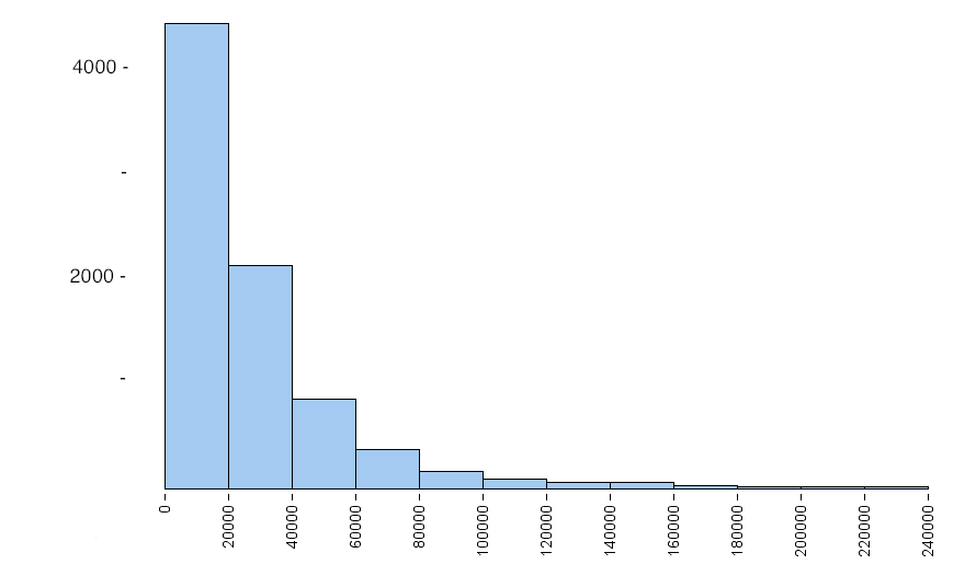
Following are some summary statistics for this data:
- Mean = $24,000, SD = $27,500
- Median = $16,900, IQR = $28,000
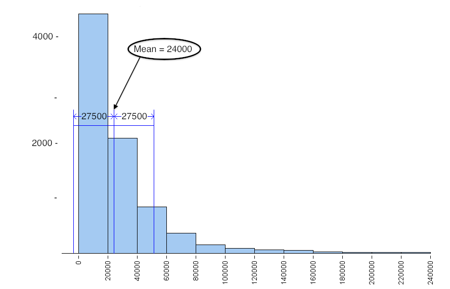
The typical range based on the mean and standard deviation is not a good summary of the distribution of incomes. The small number of people with higher incomes increases the mean. The mean is too high to represent the large number of people making less than $20,000 a year. The small number of people with higher incomes also increase the standard deviation, so a small number of high incomes gives the misleading impression that typical incomes in the sample are higher than they really are.
Notice also that Mean ± SD gives an awkward range of typical values. The left endpoint is at −3,500 (Mean − SD = 24,000 − 27,500 = −3,500), but there are no negative values in this data set. This is another reason why it is better to use the IQR when measuring the spread of a skewed data set.
Let’s take a look at the same histogram, except this time we overlay a boxplot.
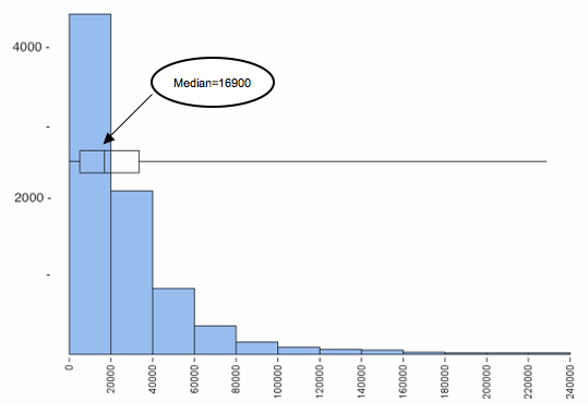
We see that the median represents the typical income of people in this sample better than the mean. The small number of people with higher incomes does not impact the median or the other quartile marks, so the first and third quartile marks give a range of incomes that more accurately represent typical incomes in the sample. Notice also that this range is always within the overall range of the data, so we will never have the problem that we encountered earlier with the standard deviation.
In a skewed distribution, the upper half and the lower half of the data have a different amount of spread, so no single number such as the standard deviation could describe the spread very well. We get a better understanding of how the values are distributed if we use the quartiles and the two extreme values in the five-number summary.
These examples illustrate some general guidelines for choosing numerical summaries:
- Use the mean and the standard deviation as measures of center and spread only for distributions that are reasonably symmetric with a central peak. When outliers are present, the mean and standard deviation are not a good choice.
- Use the five-number summary (which gives the median, IQR, and range) for all other cases.
Both of these examples also highlight another important principle: Always plot the data.
We need to use a graph to determine the shape of the distribution. By looking at the shape, we can determine which measures of center and spread best describe the data.
Let’s Summarize
- The average deviation from the mean (ADM) is a measurement of spread about the mean. More precisely, ADM measures the average distance of the data from the mean. In practice, ADM is not commonly used, but it helps us understand the standard deviation (SD).
- The standard deviation is a measure of spread. We use it as a measure of spread when we use the mean as a measure of center.
- The standard deviation is approximately the average distance of the data from the mean, so it is approximately equal to ADM.
- We can use the standard deviation to define a typical range of values about the mean. We mark the mean, then we mark 1 SD below the mean and 1 SD above the mean. This interval is centered at the mean and defines typical values about the mean. We often write this interval as Mean ± SD.
- We use technology to calculate the standard deviation.
- Like the mean, the standard deviation is strongly affected by outliers and skew in the data.
When choosing numerical summaries,
- Use the mean and the standard deviation as measures of center and spread only for distributions that are reasonably symmetric with a central peak. When outliers are present, the mean and standard deviation are not a good choice.
- Use the five-number summary (which gives the median, IQR, and range) for all other cases.
- Always plot the data. We need to use a graph to determine the shape of the distribution. By looking at the shape, we can determine which measures of center and spread best describe the data.
Candela Citations
- Concepts in Statistics. Provided by: Open Learning Initiative. Located at: http://oli.cmu.edu. License: CC BY: Attribution