Learning Objectives
- Conduct a chi-square test of independence. Interpret the conclusion in context.
In this section, we learn two new hypothesis tests: a chi-square test of independence and a chi-square test of homogeneity. As the names imply, these two tests both use the same chi-square test statistic that we learned previously to compare observed and expected counts. In addition, P-values come from the same family of chi-square distributions. Therefore, much of what we learned in the previous section, “Chi-Square Test for One-Way Tables,” will be useful here.
We begin with the chi-square test of independence. This test determines if there is a relationship between two categorical variables in the population. It is called a test of independence because “no relationship” means “independent.” If there is a relationship between the two variables in the population, then they are dependent.
We can answer the following research questions with a chi-square test of independence:
- For young adults in the United States, is gender related to body image?
- Is alcohol abuse by New York firefighters dependent on participation in the 9/11 rescue operation?
- In the United States, is race associated with political views (conservative, moderate, liberal)?
The null hypothesis states that the two categorical variables are not related in the population. In other words, the variables are independent. The alternative hypothesis says that the two categorical variables are related in the population. In other words, the variables are dependent. To test our hypotheses, we select a random sample from the population and gather data on two categorical variables from each individual. As with all chi-square tests, the expected counts reflect the null hypothesis. So we need to determine what we expect to see in a sample if the variables are independent. As before, the chi-square test statistic measures the amount that the observed counts in the sample deviate from the expected counts.
Example
Gender and Body Image
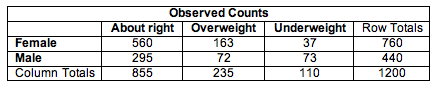
What is your perception of your own body? Do you feel that you are overweight, underweight, or about right? A random sample of 1,200 U.S. college students answered this question as part of a larger survey. The following table shows part of the responses.

Notice that the sample is a random sample from a single population: U.S. college students. Notice also that we collected data on two categorical variables for each student: gender and body image. This is the type of situation that is appropriate for a chi-square test of independence.
Step 1: State the hypotheses.
Here are two equivalent ways we can state the hypotheses for a test of independence.
- H0: There is no relationship between gender and body image for U.S. college students.
- Ha: There is a relationship between gender and body image for U.S. college students.
We could also state the hypotheses like this:
- H0: Gender and body image are independent in the population of U.S. college students.
- Ha: Gender and body image are dependent in the population of U.S. college students.
Step 2: Collect and analyze the data.
We summarized the data for this sample in a two-way table:
To investigate the relationship between gender and body image, we compare the percentage of males and females who gave each body image response. In Relationships in Categorical Data with Intro to Probability, we called these conditional percentages.
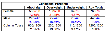
Comment: In this situation, gender is the explanatory variable. Body image is the response variable. We compare the distribution of the response variable (body image) for the groups defined by the explanatory variable (males and females). This means that explanatory category totals are the denominator of each fraction. In this case, we use male and female totals in the denominators.
We graphed these conditional percentages using ribbon charts for a visual comparison. In this sample, we can see that a larger percentage of females (73.7%) than males (67%) perceive their body weight to be “about right.” A larger percentage of females (21.4%) than males (16.4%) also perceive themselves to be overweight. Males are as likely to say they are overweight (16.4%) as underweight (16.6%), but females as much less likely to perceive themselves to be underweight (4.9%).

What do these conditional percentages have to do with independence?
Recall the definition of independence from Probability and Probability Distribution. Two events, A and B, are independent if the probability of A is the same as the probability of A when B has already occurred. We write this statement as P(A) = P(A | B). In this context, if gender and body image are independent variables, then gender does not affect the probability that a student will give a specific answer to the body image question. We use relative frequencies from the sample to represent these probabilities.
For example, we would expect the following probabilities to be the same if gender and body image are independent variables.
- P(about right) = 855/1,200 = 0.713.
- P(about right | female) = 560/760 = 0.737, which is the conditional percent shown in the ribbon chart for females.
- P(about right | male) = 295/440 = 0.67, also a conditional percent shown in the ribbon chart for males.
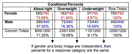
Obviously, when we compare the conditional percentages for males and females in this sample, we see that they differ. But do they differ enough to conclude that variables are dependent? Or could these results have come from a population where gender and body image are independent? In which case, the differences are due to chance fluctuation that happens in random sampling. We need to conduct a test of independence to find out.
Learn By Doing
Alcoholism Risk in 9/11 Responders
Some firefighters and other first responders to the World Trade Center on September 11, 2001, have experienced symptoms of traumatic stress, depression, anxiety, and drinking problems. Cornell University researchers conducted a survey of a random sample of New York firefighters, some of whom had participated in the 9/11 rescue efforts. The report’s title is “On the Front Line: The Work of First Responders in a Post-9/11 World.” To see the report, click here. We use data from this report to investigate the question: Are alcohol-related problems among New York firefighters associated with participation in the 9/11 rescue?
Candela Citations
- Concepts in Statistics. Provided by: Open Learning Initiative. Located at: http://oli.cmu.edu. License: CC BY: Attribution