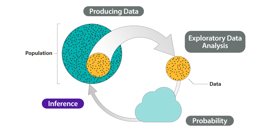
This module introduces our study of inference. Before we begin Linking Probability to Statistical Inference, let’s look at how the remainder of the course relates to the Big Picture of Statistics.
Recall that we start a statistical investigation with a research question. The investigation proceeds with the following steps:
- Produce Data: Determine what to measure, then collect the data. ← Types of Statistical Studies and Producing Data
- Explore the Data: Analyze and summarize the data. ← Summarizing Data Graphically and Numerically, Examining Relationships: Quantitative Data, Nonlinear Models, Relationships in Categorical Data with Intro to Probability
- Draw a Conclusion: Use the data, probability, and statistical inference to draw a conclusion about the population. ← Relationships in Categorical Data with Intro to Probability, Probability and Probability Distributions, Linking Probability to Statistical Inference, Inference for One Proportion, Inference for Two Proportions, Inference for Means, Chi-Square Tests
In the Big Picture of Statistics, we are about to start the last step: Inference. We use data from a sample to “infer” something about the population in this and the upcoming modules. Inference is based on probability.
Example
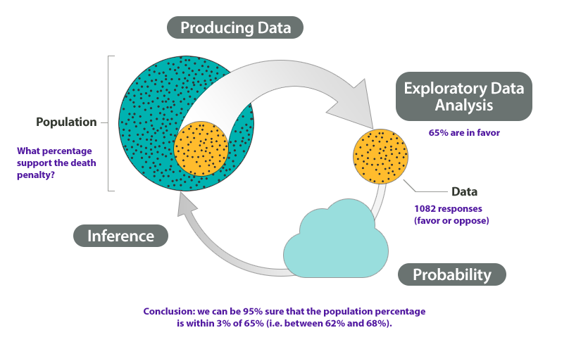
At the end of April 2005, ABC News and the Washington Post conducted a poll to determine the percentage of U.S. adults who support the death penalty.
Research question: What percentage of U.S. adults support the death penalty?
Steps in the statistical investigation:
- Produce Data: Determine what to measure, then collect the data.The poll selected 1,082 U.S. adults at random. Each adult answered this question: “Do you favor or oppose the death penalty for a person convicted of murder?”
- Explore the Data: Analyze and summarize the data.In the sample, 65% favored the death penalty.
- Draw a Conclusion: Use the data, probability, and statistical inference to draw a conclusion about the population.
Our goal is to determine the percentage of the U.S. adult population that support the death penalty. We know that different samples give different results. What are the chances that a sample reflects the opinions of the population within 3%? Probability describes the likelihood that a sample is this accurate, so we can say with 95% confidence that between 62% and 68% of the population favor the death penalty.
We illustrated the Big Picture of Statistics with an example about an inference made from survey data. From a random sample of U.S. adults, we estimated the percentage of all U.S. adults who support the death penalty. We saw that probability describes the likelihood that an estimate is within 3% of the true percentage with this opinion in the population. For this example, there is a 95% chance that a random sample is within 3% of the true population percentage.
Because random samples vary, inference always involves uncertainty. This uncertainty is captured by probability statements that are part of our conclusions. We emphasize this point in the following example where we look more closely at the process of statistical investigation with a real court case. Our goal is to identify arguments that use statistical inference to draw a conclusion as well as arguments that do not use inference.
EXAMPLE
Using Inference to Detect Cheating – A Real Case
How can a prosecutor use data to detect cheating? The details of this case appeared in Chance magazine in 1991.
The Case: During an exam at a university in Florida in 1984, the proctor suspected that one student, whom we will call Student C, was copying answers from another student, whom we will call Student A. The proctor accused Student C of cheating, and the case went to the university’s supreme court.
The Evidence: At the trial, the prosecution introduced evidence based on data. Here is the evidence: On the 16 questions missed by both Student A and Student C, 13 of the answers were the same.
The Argument: The prosecutor used the data to draw an inference based on probability. He asked the question: Could 13 out of 16 matches be due to chance? He argued that a match of 13 out of 16 by chance alone was very unlikely. The probability of this occurring is very small. So there had to be another explanation besides chance, and the prosecutor said the explanation was cheating. Based on this evidence, Student C was found guilty of academic dishonesty.
The Role of Random Chance: To decide if we agree with this argument, we need to understand if chance might explain this result. We need to determine if it would be unusual to get 13 matches on 16 questions by chance alone. To determine if 13 out of 16 is unusual, we have to look at what happens in the long run if students just guess on 16 multiple choice questions.
Let’s assume that each question had four options: a, b, c, or d. We use a computer program to randomly assign answers to each question, which mimics what happens when someone randomly guesses. Using software to imitate chance behavior is called simulation.
Here you see a representation of answers from Student A and Student C as well as three randomly generated answer sets for the 16 questions missed by both Student A and Student C. We highlighted matches with Student A’s answers in green.
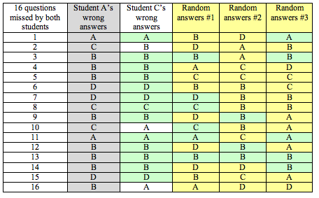
Notice that Student C has 13 answers that match Student A’s answers: As a proportion, this is 13 ÷ 16 = 0.8125. It means that about 81% of the time, Student C’s answers matched Student A’s answers on questions that they both missed.
For the random answers generated by “guessing,” we see the proportion of matches differs:
- Set 1 has 6 matches with Student A: 6 ÷ 16 = 0.375 as a proportion, or about 38%.
- Set 2 has 3 matches with Student A: 3 ÷ 16 = 0.1875 as a proportion, or about 19%.
- Set 3 has 5 matches with Student A: 5 ÷ 16 = 0.3125 as a proportion, or about 31%.
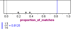
The proportion of matches in the randomly generated answers vary quite a bit, from 0.1875 to 0.3125. But none are close to the proportion of matches seen in Student C’s paper, 0.8175. The proportion of matches for the three sets of results from the random guesses are graphed in the following figure. The blue line is the proportion of matches for Student C.
Now we repeat the simulation of random sets of answers on the 16 questions, each time determining the proportion of matches to the wrong answers on Student A’s paper. On the left is a dotplot for 100 random sets of answers. Each dot represents a set of 16 answers generated by random guessing. On the right is a histogram of 1,025 random sets of answers, which shows the long-run pattern.
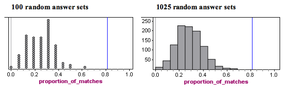
Analysis: In the histogram, we see that typical results fall between about 0.1 and 0.4. More specifically, if a student randomly guessed on these 16 questions, it would not be surprising to see from 2 to 6 matches with Student A’s wrong answers. Translated into proportions, this is 2 ÷ 16 = 0.125 to 6 ÷ 16 = 0.375.
Is Student C unusual? Yes. Notice that no randomly generated set of answers comes close to the proportion of matches on Student C’s exam. A proportion of 0.8125 would be very unusual if guessing, so we conclude that Student C was not guessing.
Conclusion: The prosecution argued that a match of 13 out of 16 wrong answers (a proportion of 0.8125) was unusual and could not be explained by random chance. Our simulation agrees with this observation. When we created answer sets by randomly guessing, we never saw more than 9 matches out of 16, which is a proportion of 0.5625. We agree with the prosecution that there has to be another explanation besides chance.
However, could there be another explanation besides cheating?
Yes. If you don’t know the answer to a question on an exam, you rarely guess at random. It is more likely that you will make an educated guess. Some wrong answers might be more logical than others. This could also explain the large proportion of matches on wrong answers between the two students. So this evidence is not convincing evidence that Student C cheated, but we know that he did not just guess.
EXAMPLE
Follow-up Argument Based on Exploratory Data Analysis
Student C appealed his case. A second trial was held. This time the prosecution made a different argument using data. This argument did not use statistical inference.
The prosecution created a new measurement. They compared every student’s paper to Student A’s paper. For the 40-multiple choice questions on the test, they counted the number of matches to Student A’s paper and divided by 40. This new measurement was also a proportion.
Analysis: There were 88 students. Here are the results:
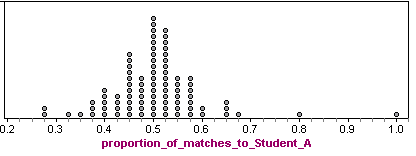
Each dot represents a student who took the exam. A dot with a proportion of 0.6 means that 60% of this student’s answers matched Student A’s answers.
Note: Student A is included in the data. Of course, Student A is the dot with the proportion of 40 out of 40 = 1.0 This makes sense because all of Student A’s answers matched Student A. (This does not mean that Student A did well on the exam.)
We see that many of the proportions fall between between 0.40 (which is 16 matches out of 40) and 0.60 (which is 24 matches out of 40). So it is not surprising if between 40% and 60% of a student’s answers matched Student A’s answers.
Student C had 32 matches out of 40, which is a proportion of 0.80. (This does not mean that Student C made an 80% on the exam. It means that 80% of Student C’s answers matched Student A’s answers.) Student C is once again an unusual data point.
Conclusion: This time it is harder to argue that Student C is not cheating. When we compare him to the rest of the class, his paper had an unusually high number of matches with Student A’s answers. This data together with the proctor’s testimony is fairly convincing evidence for the prosecution’s claim that Student C cheated by copying from Student A’s paper.
(Source: Phillip J. Boland and Michael Proschan, “The Use of Statistical Evidence in Allegations of Exam Cheating,” Chance 3(3):10-14, 1991.)
What’s the Main Point?
Statistical inference always involves an argument based on probability.
In this court case, the prosecution used two different types of arguments to provide evidence of cheating. The first argument is an example of statistical inference because it is based on probability. We set up a simulation to reflect an assumption that the prosecutor made. The assumption is that answer sets come from random guessing. We simulated over a thousand answer sets with randomly chosen answers to investigate the long-run behavior of simulated answer sets. We then compared Student C to the distribution of randomly generated answer sets. Student C was unusual. We concluded that Student C was not randomly guessing.
The second argument is an example of exploratory data analysis with no statistical inference. The prosecutor designed a measurement and collected data from every student in the class. He compared Student C’s measurement to the measurements of the other students. Probability did not have a role in this analysis. Probability statements require a random event and a look at long-run behavior of random events, so this is not an example of statistical inference.
LEARN BY DOING
LEARN BY DOING
The court case illustrates how we can view statistical inference as an argument based on probability. Here we briefly connect the probability argument with the vocabulary and ideas from the module Probability and Probability Distribution.
Recall the following important points about probability that we learned in that module:
- Probability is a measure of how likely an event is to occur.
- We can make probability statements only about random events. Random here means that the outcome is uncertain in the short run but has a predictable pattern in the long run.
How does the logic of the probability argument in the court case relate to Probability and Probability Distribution?
To understand the probability argument in the original court case, we used a computer simulation to analyze the long-run pattern that emerges if students randomly guess on multiple-choice questions. Our variable was Proportion of matches with Student A’s wrong answers on 16 questions. We graphed the distribution of a large number of proportions from the random answer sets to see the pattern. Using the vocabulary of Probability and Probability Distribution, the proportion of matches is a random variable. In the short run, we do not know the proportion of matches that will occur in a random answer set, but in the long run, we see a pattern in the distribution of these proportions. This distribution of proportions is treated as a probability model. From it we can see how much variability to expect in matches from random answer sets. We can also identify unusual values. From the pattern in this distribution, we can say it is very unlikely that Student C guessed.
How does this logic relate to the Big Picture?
This logic is similar to the logic of inference that we explore in future modules, where we randomly select samples from a population. We continue to use computer simulation throughout these modules to analyze the long-run pattern that emerges in measurements from random samples. We create probability models that tell us how much variability to expect in random samples. We also use these models to identify unusual measurements. From the patterns, we use data to make judgments about the population. In this way, our conclusions about a population are based on probability.
Probability and Probability Distribution included a long discussion of probability models that are normal curves. Under certain conditions, the long-run behavior of measurements from random samples can be modeled with a normal curve (or a similar curve), we see in this module and in Inference for One Proportion, Inference for Two Proportions, and Inference for Means. In each module, we ask the question, When can we use a normal model? Once we know these conditions, we can use what we learned in the previous module to make probability-based decisions about population values.
Here we add these ideas to the Big Picture to show how probability connects to inference.
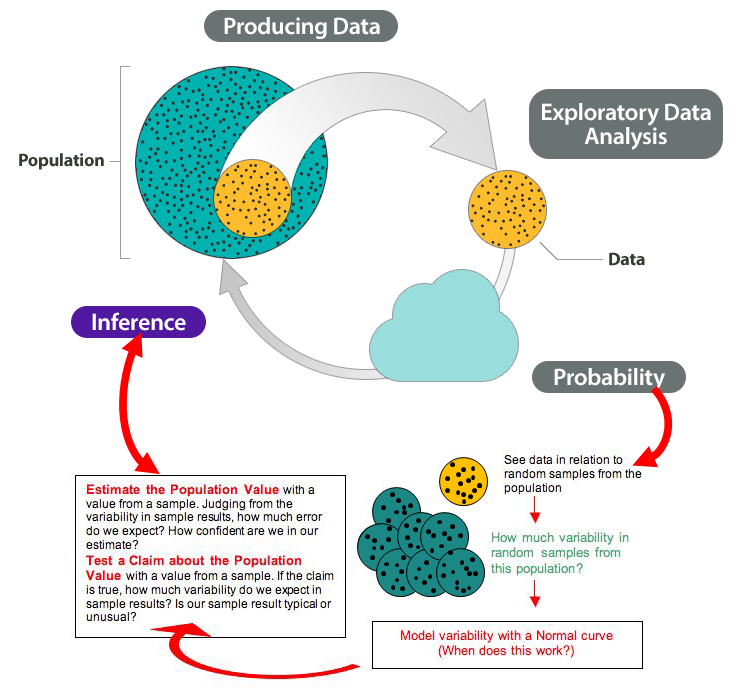
Note that we highlighted two types of inference in the diagram:
- Estimate a population value.
- Test a claim about the population value.
We end our introduction to inference with a look at research questions that illustrate these two types of inference. We also connect these examples to the types of inference we learn about in upcoming modules.
Research Questions That Involve Inference
| Type of Question | Examples | Variable Type | Unit |
|---|---|---|---|
| Make an estimate about the population | What proportion of all U.S. adults support the death penalty? | Categorical variable | Inference for One Proportion |
| What is the average number of hours that community college students work each week? | Quantitative variable | Inference for Means | |
| Test a claim about the population | Do the majority of community college students qualify for federal student loans? | Categorical variable | Inference for One Proportion |
| Has the average birth weight in a town decreased from 3,500 grams? | Quantitative variable | Inference for Means | |
| Compare two populations | Are teenage girls more likely to suffer from depression than teenage boys? | Categorical variable | Inference for Two Proportions |
| In community colleges do female students have a higher average GPA than male students? | Quantitative variable | Inference for Means |
Note: Each research question relates to either a categorical variable or a quantitative variable. In this course, three criteria determine the inference procedure we use:
- The type of variable.
- The type of inference (estimate a population value or test a claim about a population value).
- The number of populations involved.
LEARN BY DOING
Candela Citations
- Concepts in Statistics. Provided by: Open Learning Initiative. Located at: http://oli.cmu.edu. License: CC BY: Attribution