Kinematics
Concepts and Principles
Kinematics is the formal language physicists use to describe motion. The need for a formal language is evidenced by a simple experiment: drop an object from about shoulder height and ask two people to independently describe the motion of the object. Chances are that the descriptions will not be in perfect agreement, even though both observers described the same motion. Obviously, a more formal way of describing motion is necessary to eliminate this type of descriptive ambiguity. Kinematics is the formal method of describing motion.
Three parameters are carefully defined and used by physicists to describe motion. Specifying these three parameters at all times forms a complete description of the motion of an object.
Position
The position of an object is its location relative to a well-defined coordinate system at a particular instant of time. Without a specified coordinate system, position is a meaningless concept. A coordinate system is comprised of a zero, a specified positive direction, and a scale.
For example, in the hypothetical experiment in which the object was dropped from shoulder height, a coordinate system could have been defined in which the zero position was at ground level, the positive direction was up, and the scale used was meters. Using this coordinate system, the position of the object could have been specified at any particular instant of time. Of course, choosing the zero at the location at which the object was dropped, the positive direction as down, and the scale in feet is also perfectly acceptable. It doesn’t matter what you choose as a coordinate system, only that you explicitly choose one. Depending on the coordinate system chosen, the position of an object can be positive, negative, or zero.
We will use the symbol r to designate position, and measure it in meters (m).
Velocity
Although the word velocity is often used loosely in everyday conversation, its meaning in physics is specific and well-defined. To physicists, the velocity is the rate at which the position is changing. The velocity can be specified at any particular instant of time.
For example, if the position is changing quickly the velocity is large and if the position is not changing at all the velocity is zero. A mathematical way to represent this definition is
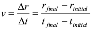
Thus, velocity is measured in meters per second (m/s).
Actually, this is the definition of the average velocity of the object over the time interval Dt, but as the time interval becomes smaller and smaller the value of this expression becomes closer and closer to the actual rate at which the position is changing at one particular instant of time.
Since the final position of the object (rfinal) may be either positive, negative, or zero, and either larger, smaller, or the same as the initial position (rinitial), the velocity may be positive, negative, or zero. The sign of the velocity depends on the coordinate system chosen to define the position. A positive velocity simply means that the object is moving in the positive direction, as defined by the coordinate system, while a negative velocity means the object is traveling in the other direction.
Acceleration
Again, although the word acceleration is often used loosely in everyday conversation, its meaning in physics is specific and well-defined. To physicists, the acceleration is the rate at which the velocity is changing. Again, the acceleration can be specified at any particular instant of time.
For example, if the velocity is changing quickly the acceleration is large in magnitude, and if the velocity is not changing the acceleration is zero. If an object has non-zero acceleration, it does not mean that the object is speeding up. It simply means that the velocity is changing. Moreover, even if an object has a positive acceleration, it does not mean that the object is speeding up! A positive acceleration means that the change in the velocity points in the positive direction. (I can almost guarantee you will experience confusion about this. Take some time to think about the preceding statement right now.)
A mathematical way to represent acceleration is
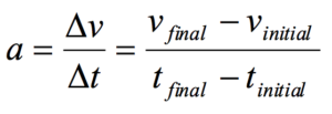
Thus, acceleration is measured in meters per second per second (m/s2).
Again, this is actually the average acceleration of the object over the time interval Dt, but as the time interval becomes smaller and smaller, the value of this expression becomes closer and closer to the actual rate at which the velocity is changing at one particular instant of time.
Since vfinal may be either positive, negative, or zero, and either larger, smaller, or the same as vinitial, the acceleration may be positive, negative, or zero. The algebraic sign of the acceleration depends on the coordinate system chosen to define the position. A negative acceleration means that the change in the velocity points in the negative direction. For example, the velocity could be in the positive direction and the object slowing down or the velocity could be in the negative direction and the object speeding up. Both of these scenarios would result in a negative acceleration. Conversely, a positive acceleration means that the change in the velocity points in the positive direction.
Kinematics is the correct use of the parameters position, velocity, and acceleration to describe motion. Learning to use these three terms correctly can be made much easier by learning a few tricks of the trade. These tricks, or analysis tools, are detailed in the following section.
Analysis Tools
Drawing Motion Diagrams
The words used by physicists to describe the motion of objects are defined above. However learning to use these terms correctly is more difficult than simply memorizing definitions. An extremely useful tool for bridging the gap between a normal, conversational description of a situation and a physicists’ description is the motion diagram. A motion diagram is the first step in translating a verbal description of a phenomenon into a physicists’ description.
Start with the following verbal description of a physical situation:
The driver of an automobile traveling at 15 m/s, noticing a red-light 30 m ahead, applies the brakes of her car until she stops just short of the intersection.
Determining the position from a motion diagram
A motion diagram can be thought of as a multiple-exposure photograph of the physical situation, with the image of the object displayed at equal time intervals. For example, a multiple-exposure photograph of the situation described above would look something like this:

Note that the images of the automobile are getting closer together near the end of its motion because the car is traveling a smaller distance between the equally-timed exposures.
In general, in drawing motion diagrams it is better to represent the object as simply a dot, unless the actual shape of the object conveys some interesting information. Thus, a better motion diagram would be:

Since the purpose of the motion diagram is to help us describe the car’s motion, a coordinate system is necessary. Remember, to define a coordinate system you must choose a zero, define a positive direction, and select a scale. We will always use meters as our position scale in this course, so you must only select a zero and a positive direction. Remember, there is no correct answer. Any coordinate system is as correct as any other.
The choice below indicates that the initial position of the car is the origin, and positions to the right of that are positive. (In the text I’ll always use a little diamond to indicate the zero with an arrow pointing in the positive direction.)

We can now describe the position of the car. The car starts at position zero and then has positive, increasing positions throughout the remainder of its motion.
Determining the velocity from a motion diagram
Since velocity is the change in position of the car during a corresponding time interval, and we are free to select the time interval as the time interval between exposures on our multiple-exposure photograph, the velocity is simply the change in the position of the car “between dots.” Thus, the arrows (vectors) on the motion diagram below represent the velocity of the car.

We can now describe the velocity of the car. Since the velocity vectors always point in the positive direction, the velocity is always positive. The car starts with a large, positive velocity which gradually declines until the velocity of the car is zero at the end of its motion.
Determining the acceleration from a motion diagram
Since acceleration is the change in velocity of the car during a corresponding time interval, and we are free to select the time interval as the time interval between exposures on our multiple-exposure photograph, we can determine the acceleration by comparing two successive velocities. The change in these velocity vectors will represent the acceleration.
To determine the acceleration,
- select two successive velocity vectors,
- draw them starting from the same point,
- construct the vector (arrow) that connects the tip of the first velocity vector to the tip of the second velocity vector.
- The vector you have constructed represents the acceleration.
Comparing the first and second velocity vectors leads to the acceleration vector shown below:

Thus, the acceleration points to the left and is therefore negative. You could construct the acceleration vector at every point in time, but hopefully you can see that as long as the velocity vectors continue to point toward the right and decrease in magnitude, the acceleration will remain negative.
Thus, with the help of a motion diagram, you can extract lots of information about the position, velocity, and acceleration of an object. You are well on your way to a complete kinematic description.
Drawing Motion Graphs
Another useful way to describe the motion of an object is by constructing graphs of the object’s position, velocity, and acceleration vs. time. A graphical representation is a very effective means of presenting information concerning an object’s motion and, moreover, it is relatively easy to construct motion graphs if you have a correct motion diagram.
Examine the same situation as before:
The driver of an automobile traveling at 15 m/s, noticing a red-light 30 m ahead, applies the brakes of her car until she stops just short of the intersection.

The verbal representation of the situation has already been translated into a motion diagram. A careful reading of the motion diagram allows the construction of the motion graphs.
Drawing the position vs. time graph
We already know, from the motion diagram, that the car starts at position zero, then has positive, increasing positions throughout the remainder of its motion. This information can be transferred onto a position vs. time graph.
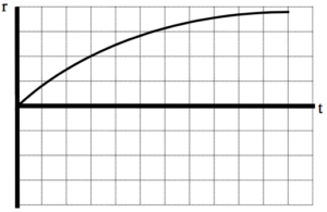
Notice that the position is zero when the time is equal to zero, the position is always positive, and the position increases as time increases. Also note that in each subsequent second, the car changes its position by a smaller amount. This leads to the graph of position vs. time gradually decreasing in slope until it achieves a slope of zero. Once the car stops, the position of the car should not change.
Drawing the velocity vs. time graph
From the motion diagram, we know that the velocity of the car is always positive, starts large in magnitude, and decreases until it is zero. This information can be transferred onto a velocity vs. time graph.
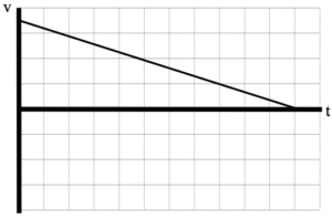
How do we know that the slope of the line is constant? The slope of the line represents the rate at which the velocity is changing, and the rate at which the velocity is changing is termed the acceleration. Since in this model of mechanics we will only consider particles undergoing constant acceleration, the slope of a line on a velocity vs. time graph must be constant.
Drawing the acceleration vs. time graph
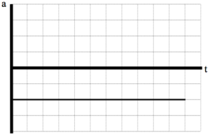
From the motion diagram, the acceleration of the car can be determined to be negative at every point. Again, in this pass through mechanics we will only be investigating scenarios in which the acceleration is constant. Thus, a correct acceleration vs. time graph is shown below.
Tabulating Motion Information
After constructing the two qualitative representations of the motion (the motion diagram and the motion graphs), we are ready to tackle the quantitative aspects of the motion.
Utilizing the motion diagram,

you can now assign numerical values to several of the kinematic variables. A glance at the situation description should indicate that information is presented about the car at two distinct events. Information is available about the car at the instant the driver applies the brakes (the velocity is given), and the instant the driver stops (the position is given). Other information can also be determined by referencing the motion diagram. To tabulate this information, you should construct a motion table.
| Event 1: The instant the driver first applies the brakes.
t1 = 0 s r1 = 0 m v1 = +15 m/s a12 = |
Event 2: The instant the car finally stops.
t2 = r2 = +30 m v2 = 0 m/s |
In addition to the information explicitly given, the velocity at the first event and the position at the second event, other information can be extracted from the problem statement and the motion diagram.
For example,
- the position of the car at the first event is zero because the origin of the coordinate system is at this point,
- the time at the first instant can be “set to zero” by imagining a hypothetical stopwatch that is clicked on as the car begins to brake,
- and the velocity at the second event is zero because the car is stopped.
Since you are working under the assumption in this model that the acceleration is constant, the acceleration between the two instants in time is some unknown, constant value. To remind you that this assumption is in place, the acceleration is not labeled at the first instant, a1, or the second instant, a2, but rather as the acceleration between the two instants in time, a12.
You now have a complete tabulation of all the information presented, both explicitly and implicitly, in the situation description. Moreover, you now can easily see that the only kinematic information not known about the situation is the assumed constant acceleration of the auto and the time at which it finally stops. Thus, to complete a kinematic description of the situation these two quantities must be determined. What you may not know is that you have already been presented with the information needed to determine these two unknowns.
Doing the Math
In the concepts and principles portion of this unit, you were presented with two formal, mathematical relationships, the definitions of velocity and acceleration. In the example that you are working on, there are two unknown kinematic quantities. You should remember from algebra that two equations are sufficient to calculate two unknowns. Thus, by applying the two definitions you should be able to determine the acceleration of the car and the time at which it comes to rest.
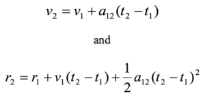
Although you can simply apply the two definitions directly, normally the two definitions are rewritten, after some algebraic re-arranging, into two different relationships. This rearrangement is simply to make the algebra involved in solving for the unknowns easier. It is by no means necessary to solve the problem. In fact, the two definitions can be written in a large number of different ways, although this does not mean that there are a large number of different formulas you must memorize in order to analyze kinematic situations. There are only two independent kinematic relationships. The two kinematic relationships[1] we will use when the acceleration is constant are:
To finish the analysis of this situation,
| Event 1: The instant the driver first applies the brakes.
t1 = 0 s r1 = 0 m v1 = +15 m/s a12 = |
Event 2: The instant the car finally stops.
t2 = r2 = +30 m v2 = 0 m/s |
simply write the two kinematic relationships, input the known kinematic variables from the motion table, and solve the two relations for the two unknowns. (This process is not physics, it’s algebra.)

Now substitute this expression into the other equation:
|

Substitute this result back into the original equation: |
Thus, the car must have accelerated at 3.8 m/s2 in the negative direction, and stopped after 4.0 seconds. The kinematic description of the situation is complete.
Analyzing a More Complex Motion
Let’s re-visit our scenario, although this time the light turns green while the car is slowing down:
The driver of an automobile traveling at 15 m/s, noticing a red-light 30 m ahead, applies the brakes of her car. When she is 10 m from the light, and traveling at 8.0 m/s, the light turns green. She instantly steps on the gas and is back at her original speed as she passes under the light.
Our first step in analyzing this motion should be to draw a motion diagram.

I’ve noted on the motion diagram the important events that take place during the motion. Notice that between the instant she hits the brakes and the instant she steps on the gas the acceleration is negative, while between the instant she steps on the gas and the instant she passes the light the acceleration is positive. Thus, in tabulating the motion information and applying the kinematic relations we will have to be careful not to confuse kinematic variables between these two intervals. Below is a tabulation of motion information using the coordinate system established in the motion diagram.
| Event 1: She hits the brakes.
t1 = 0 s r1 = 0 m v1 = +15 m/s a12 = |
Event 2: She steps on the gas.
t2 = r2 = +20 m v2 = +8.0 m/s a23 = |
Event 3: She passes the light
t3 = r3 = +30 m v3 = +15 m/s |
First, notice that during the time interval between “hitting the brakes” and “stepping on the gas” there are two kinematic variables that are unknown. Recall that by using your two kinematic relations you should be able to determine these values. Second, notice that during the second time interval again two variables are unknown. Once again, the two kinematic relations will allow you to determine these values. Thus, before I actually begin to do the algebra I know the unknown variables can be determined!
First let’s examine the motion between hitting the brakes and stepping on the gas:

Now substitute this expression into the other equation:
|

Substitute this result back into the original equation: |
Now, using these results, examine the kinematics between stepping on the gas and passing the light. Note that the initial values of the kinematic variables are denoted by ‘2’ and the final values by ‘3’, since we are examining the interval between event 2 and event 3.

Now substitute this expression into the other equation:
|

Substitute this result back into the original equation:
|
We now have a complete kinematic description of the motion.
Symbolic Analysis
Consider the following situation:
The driver of an automobile suddenly sees an obstacle blocking her lane. Determine the total distance the auto travels between seeing the obstacle and stopping (d) as a function of the initial velocity of the car (vi) and the magnitude of its acceleration while stopping (as).
As always, the first step in analyzing motion is to draw a motion diagram.

Rather than calculate the stopping distance for particular values of initial velocity and acceleration, the goal of this activity is to determine, in general, how the stopping distance depends on these two parameters. If we can construct this function we can then use the result to calculate the stopping distance for any car if we know its initial velocity and stopping acceleration.
Although this sounds like a different task from what we’ve done in the previous two examples we will approach this task exactly the same way, by tabulating what we know about the situation,
| Event 1: The instant the driver hits the brakes.
t1 = 0 s r1 = 0 m v1 = vi a12 = -as |
Event 2: The instant the car stops.
t2 = r2 = d v2 = 0 m/s |
and then applying our two kinematic relationships:

Since our goal is to determine d as a function of vi and as, we must eliminate t2. To do this, solve for t2 in the left equation and substitute this expression into the right equation.
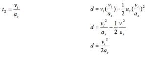
Thus, the stopping distance appears to be proportional to the square of the initial velocity and inversely proportional to the stopping acceleration. Does this make sense?
To determine if a symbolic expression is sensible it is often useful to check limiting cases. A limiting case is when one of the variables in the expression takes on an extreme value, typically zero or infinity. For example, if the initial velocity of the car was zero the stopping distance would have to also be zero, since the car was never moving! Allowing vi to equal zero in the above expression results in a stopping distance of zero, so our expression “passes” this logical test.
Another limiting case would be setting the acceleration of the car equal to zero. With no acceleration, the car should never stop. In our expression, setting the acceleration equal to zero results in an infinite stopping distance, which again agrees with commonsense. If our expression didn’t give the correct results in these limiting cases we would know we made an error somewhere in the derivation (and, of course, we would then go back and find our mistake and fix it because we are good students …).
Hints and Suggestions
Algebraic Signs
Confusion about the meaning of algebraic signs is common among beginning physics students. The best way to clarify this confusion is to remember that algebraic signs are simply a mathematical way to describe direction. Instead of saying up and down, or east and west, physicists construct coordinate systems and translate the words east and west into the symbols ‘+’ and ‘-’, or even ‘-’ and ‘+’ if we choose a different coordinate system. The key to the translation is the coordinate system. A coordinate system is very similar to the English-French dictionary you might take with you on your first trip to France. When you see a ‘-’, use your coordinate system to translate it into a verbal description of direction.
Do not fall into the common habit of translating a ‘-’ into the word “decreasing”. A negative acceleration, for example, does NOT imply that the object is slowing down. It implies an acceleration that points in the negative direction. It is impossible to determine whether an object is speeding up or slowing down by looking at the sign of the acceleration! Conversely, the word “deceleration”, which does mean that an object is slowing down, does not give any information regarding the sign of the acceleration. I can decelerate in the positive direction as easily as I can decelerate in the negative direction.
Addendum
Deriving the kinematic relationships
Let’s construct the two independent kinematic relationships that you will use whenever the acceleration is constant. In a later chapter, we will return to the case in which the acceleration is not constant.
From the definition of acceleration:
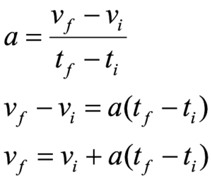
The above relationship is our first kinematic relationship. The acceleration in this relationship is really the average acceleration. However, since the acceleration is constant in this model the average acceleration is the same as the acceleration at any instant between the initial and final state.
From the definition of velocity:
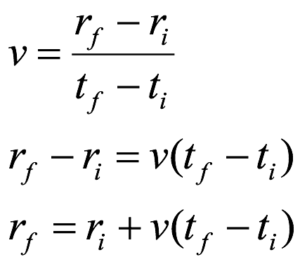
You must remember, however, that the velocity in this formula is really the average velocity of the object over the time interval selected. To keep you from having to remember this fact, we can rewrite the average velocity as the sum of the initial velocity and the final velocity divided by two:

Substituting in the first kinematic relationship for the final velocity yields:
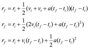
The above relationship is our second kinematic relationship.
Although we could keep deriving new kinematic equations forever, it is impossible that any other derived equation could allow us to calculate some quantity that these equations do not allow us to calculate.
Activities
Construct motion diagrams for the motions described below on a separate piece of paper.
a. A subway train in Washington, D.C., starts from rest and accelerates at 2.0 m/s2 for 12 seconds.
b. The driver of a car traveling at 35m/s suddenly sees a police car. The driver attempts to reach the speed limit of 25 m/s by accelerating at 2.5 m/s2. The driver has a reaction time of 0.55 s. (The reaction time is the time between first seeing the police car and pressing the brake.)
c. A pole-vaulter, just before touching the cushion on which she lands after a jump, is falling downward at a speed of 10 m/s. The pole-vaulter sinks about 2.0 m into the cushion before stopping.
d. An elevator is moving downward at 4.0 m/s for 3.5 s before someone presses the emergency stop button. The elevator comes to rest after traveling 2.9 m.
Construct motion diagrams for the motions described below.
a. An automobile comes to rest after skidding 35 m. The car’s acceleration while skidding is known to be 6.0 m/s2.
b. A car, initially traveling at 20 m/s to the east, accelerates toward the west at 2.0 m/s2. At the same time that the car starts moving, a truck, 60 m west of the car and moving at 16 m/s toward the east, starts to move faster, accelerating at 1.0 m/s2. It’s a one-lane road and both drivers are too busy texting to notice each other.
c. A child is hanging from a rope by her hands. She exerts a burst of strength and 2.0 s later is traveling at 1.4 m/s up the rope.
d. A two-stage rocket initially accelerates upward from rest at 13 m/s2 for 5.0s before the second stage initiates a 14 s long upward acceleration of 25 m/s2.
For each of the motion diagrams below, determine the algebraic sign (+, – or zero) of the position, velocity, and acceleration of the object at the location of the three open circles. Describe an actual motion that could be represented by each motion diagram.
a. 
Description:
| 1 | 2 | 3 | |
| r | |||
| v | |||
| a |
b.
Description:
| 1 | 2 | 3 | |
| r | |||
| v | |||
| a |
c.
Description:
| 1 | 2 | 3 | |
| r | |||
| v | |||
| a |
For each of the motion diagrams below, determine the algebraic sign (+, – or zero) of the position, velocity, and acceleration of the object at the location of the three open circles. Describe an actual motion that could be represented by each motion diagram.
a. 
Description:
| 1 | 2 | 3 | |
| r | |||
| v | |||
| a |
b.
Description:
| 1 | 2 | 3 | |
| r | |||
| v | |||
| a |
c.
Description:
| 1 | 2 | 3 | |
| r | |||
| v | |||
| a |
For each of the position vs. time graphs below, construct a corresponding motion diagram and velocity vs. time graph.
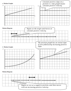
For each of the position vs. time graphs below, construct a corresponding motion diagram and velocity vs. time graph.
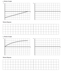
For each of the graphs below, construct a corresponding graph and motion diagram.
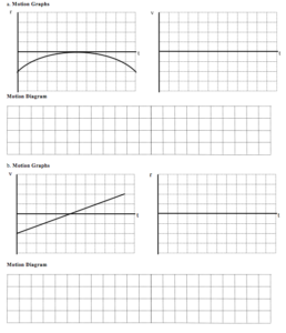
For each of the graphs below, construct a corresponding graph and motion diagram.
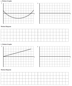
For each of the motion diagrams below, construct the corresponding motion graphs.
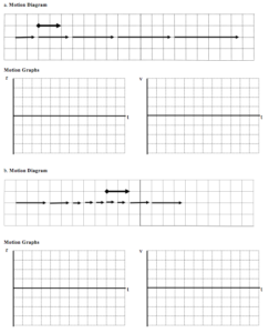
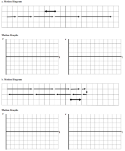
For each of the motion diagrams below, construct the corresponding motion graphs.
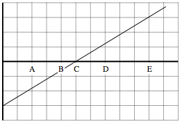
An object’s motion is represented by the position vs. time graph above.
a. Rank the object’s position at the lettered times.
Largest Positive 1. E 2. D 3. C 4. B 5. A Largest Negative
b. Rank the object’s velocity at the lettered times.
Largest Positive 1. ABCDE 2. 3. 4. 5. Largest Negative
Constant slope means constant velocity (and zero acceleration)
c. Rank the object’s acceleration at the lettered times.
Largest Positive 1. 2. 3. ABCDE 4. 5. Largest Negative
An object’s motion is represented by the velocity vs. time graph above.
d. Rank the object’s position at the lettered times.
Largest Positive 1. E 2. A 3. D 4. B 5. C Largest Negative
The motion diagram for the object is sketched below. Notice that regardless of where the origin is located, the turn-around point (C) is the smallest position.

e. Rank the object’s velocity at the lettered times.
Largest Positive 1. E 2. D 3. C 4. B 5. A Largest Negative
f. Rank the object’s acceleration at the lettered times.
Largest Positive 1. ABCDE 2. 3. 4. 5. Largest Negative
Constant slope means constant acceleration.
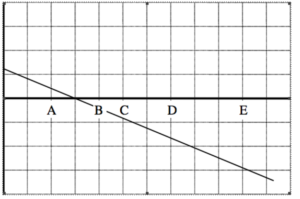
An object’s motion is represented by the position vs. time graph above.
a. Rank the object’s position at the lettered times.
Largest Positive 1. _____ 2. _____ 3. _____ 4. _____ 5. _____ Largest Negative
b. Rank the object’s velocity at the lettered times.
Largest Positive 1. _____ 2. _____ 3. _____ 4. _____ 5. _____ Largest Negative
c. Rank the object’s acceleration at the lettered times.
Largest Positive 1. _____ 2. _____ 3. _____ 4. _____ 5. _____ Largest Negative
An object’s motion is represented by the velocity vs. time graph above.
a. Rank the object’s position at the lettered times.
Largest Positive 1. _____ 2. _____ 3. _____ 4. _____ 5. _____ Largest Negative
b. Rank the object’s velocity at the lettered times.
Largest Positive 1. _____ 2. _____ 3. _____ 4. _____ 5. _____ Largest Negative
c. Rank the object’s acceleration at the lettered times.
Largest Positive 1. _____ 2. _____ 3. _____ 4. _____ 5. _____ Largest Negative
 An object’s motion is represented by the position vs. time graph at right.
a. Rank the object’s position at the lettered times.
Largest Largest
Positive Negative
1. _____ 2. _____ 3. _____ 4. _____ 5. _____
b. Rank the object’s velocity at the lettered times.
Largest Largest
Positive Negative
1. _____ 2. _____ 3. _____ 4. _____ 5. _____
c. Rank the object’s acceleration at the lettered times.
Largest Largest
Positive Negative
1. _____ 2. _____ 3. _____ 4. _____ 5. _____
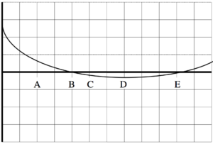
An object’s motion is represented by the position vs. time graph at right.
d. Rank the object’s position at the lettered times.
Largest Largest
Positive Negative
1. _____ 2. _____ 3. _____ 4. _____ 5. _____
e. Rank the object’s velocity at the lettered times.
Largest Largest
Positive Negative
1. _____ 2. _____ 3. _____ 4. _____ 5. _____
f. Rank the object’s acceleration at the lettered times.
Largest Largest
Positive Negative
1. _____ 2. _____ 3. _____ 4. _____ 5. _____
 An object’s motion is represented by the position vs. time graph at right.
a. Rank the object’s position at the lettered times.
Largest Largest
Positive Negative
1. _____ 2. _____ 3. _____ 4. _____ 5. _____
b. Rank the object’s velocity at the lettered times.
Largest Largest
Positive Negative
1. _____ 2. _____ 3. _____ 4. _____ 5. _____
c. Rank the object’s acceleration at the lettered times.
Largest Largest
Positive Negative
1. _____ 2. _____ 3. _____ 4. _____ 5. _____
 An object’s motion is represented by the position vs. time graph at right.
d. Rank the object’s position at the lettered times.
Largest Largest
Positive Negative
1. _____ 2. _____ 3. _____ 4. _____ 5. _____
e. Rank the object’s velocity at the lettered times.
Largest Largest
Positive Negative
1. _____ 2. _____ 3. _____ 4. _____ 5. _____
f. Rank the object’s acceleration at the lettered times.
Largest Largest
Positive Negative
1. _____ 2. _____ 3. _____ 4. _____ 5. _____
Below are velocity vs. time graphs for six different objects.
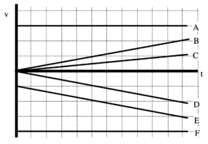
Rank these graphs on the basis of the distance traveled by each object.
Largest 1. ___F___ 2. ___A___ 3. ___E___ 4. ___B D___ 5. ___C___ 6. _____ Smallest
_____ The ranking cannot be determined based on the information provided.
Explain the reason for your ranking:
The faster you travel, the more distance you travel. The direction you are headed is not important. Therefore, F travels the largest distance because it is always moving the fastest, followed by A. E is consistently traveling faster than D, so it covers a larger distance than D. B and D always travel at the same speed (although in opposite directions) so they cover the same distance, therefore they are ranked as equal. C travels the slowest so it covers the least distance.
Below are position vs. time graphs for six different objects.
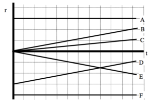
- Rank these graphs on the basis of the velocity of the object.
Largest Positive 1. _____ 2. _____ 3. _____ 4. _____ 5. _____ 6. _____ Largest Negative
_____ The ranking cannot be determined based on the information provided.
Explain the reason for your ranking:
- Rank these graphs on the basis of the acceleration of the object.
Largest Positive 1. _____ 2. _____ 3. _____ 4. _____ 5. _____ 6. _____ Largest Negative
_____ The ranking cannot be determined based on the information provided.
Explain the reason for your ranking:
Below are velocity vs. time graphs for six different objects.

- Rank these graphs on the basis of the final position of each object.
Largest Positive 1. _____ 2. _____ 3. _____ 4. _____ 5. _____ 6. _____ Largest Negative
_____ The ranking cannot be determined based on the information provided.
Explain the reason for your ranking:
- Rank these graphs on the basis of the acceleration of the object.
Largest Positive 1. _____ 2. _____ 3. _____ 4. _____ 5. _____ 6. _____ Largest Negative
_____ The ranking cannot be determined based on the information provided.
Explain the reason for your ranking:
A pole-vaulter, just before touching the cushion on which she lands after a jump, is falling downward at a speed of 10 m/s. The pole-vaulter sinks about 2.0 m into the cushion before stopping.

A child is hanging from a rope by her hands. She exerts a burst of strength and 2.0 s later is traveling at 1.4 m/s up the rope.
Motion Diagram Motion Information
| Event 1:
t1 = r1 = v1 = a12 =
|
Event 2:
t2 = r2 = v2 =
|
Mathematical Analysis
An elevator is moving downward at 4.0 m/s when someone presses the emergency stop button. The elevator comes to rest after traveling 2.9 m.
Motion Diagram Motion Information
| Event 1:
t1 = r1 = v1 = a12 =
|
Event 2:
t2 = r2 = v2 =
|
Mathematical Analysis
The driver of a car traveling at 16 m/s suddenly sees a truck that has entered from a side street and blocks the car’s path. The car’s maximum magnitude acceleration while braking is 6.0 m/s2 and the driver has a reaction time of 0.75 s. (The reaction time is the time between first seeing the truck and pressing the brake.) The driver stops just in time to avoid an accident.
Motion Diagram
Motion Information
| Event 1:
t1 = r1 = v1 = a12 = |
Event 2:
t2 = r2 = v2 = a23 = |
Event 3:
t3 = r3 = v3 =
|
Mathematical Analysis
The driver of a car traveling at 35 m/s suddenly sees a police car. The driver attempts to reach the speed limit of 25 m/s by accelerating at 2.5 m/s2. The driver has a reaction time of 0.55 s. (The reaction time is the time between first seeing the police car and pressing the brake.)
Motion Diagram
Motion Information
| Event 1:
t1 = r1 = v1 = a12 = |
Event 2:
t2 = r2 = v2 = a23 = |
Event 3:
t3 = r3 = v3 =
|
Mathematical Analysis
An automobile, initially traveling at 15 m/s, begins to slow down as it approaches a red light. After traveling 15 m, and slowing to 3.0 m/s, the light turns green and the driver steps on the gas and accelerates for 2.4 seconds until she reaches her original speed.
Motion Diagram
Motion Information
| Event 1:
t1 = r1 = v1 = a12 = |
Event 2:
t2 = r2 = v2 = a23 = |
Event 3:
t3 = r3 = v3 =
|
Mathematical Analysis
A two-stage rocket initially accelerates upward from rest at 13 m/s2 for 5.0s before the second stage ignites. The second stage “burns” for 14 s and results in the rocket achieving a speed of 415 m/s at the end of this stage.
Motion Diagram Motion Information
| Event 1:
t1 = r1 = v1 = a12 =
|
Event 2:
t2 = r2 = v2 = a23 =
|
Event 3:
t3 = r3 = v3 =
|
Mathematical Analysis
Rather than pushing the button for the correct floor a man prefers to hit the emergency stop button when an elevator approaches his floor, and then pry the doors apart. An elevator is moving at a constant speed of 2.8 m/s when it is 16 m from his floor. With uncanny timing, and an elevator that can slow at 3.5 m/s2, he makes the elevator stop precisely at his floor.
Motion Diagram Motion Information
| Event 1:
t1 = r1 = v1 = a12 =
|
Event 2:
t2 = r2 = v2 = a23 =
|
Event 3:
t3 = r3 = v3 =
|
Mathematical Analysis
A subway train in Washington, D.C., starts from rest and accelerates at 2.0 m/s2 for 12 s. The train travels at a constant speed for 65 s. The speed of the train then decreases for 25 s until it reaches the next station.
Motion Diagram
Motion Information
| Event 1:
t1 = r1 = v1 = a12 = |
Event 2:
t2 = r2 = v2 = a23 = |
Event 3:
t3 = r3 = v3 = a34 = |
Event 4:
t4 = r4 = v4 = |
Mathematical Analysis
A rocket ship is launched from rest from a space station. Its destination is 1.0 x 10¹¹ m away. The ship is programmed to accelerate at 7.4 m/s2 for 12 hours. After 12 hours, the ship will travel at constant velocity until it comes within 1.0 x 10¹⁰ m of its destination. Then, it will fire its retrorockets to land safely.
Motion Diagram
Motion Information
| Event 1:
t1 = r1 = v1 = a12 = |
Event 2:
t2 = r2 = v2 = a23 = |
Event 3:
t3 = r3 = v3 = a34 = |
Event 4:
t4 = r4 = v4 = |
Mathematical Analysis
The driver of a car traveling at 16 m/s sees a truck 20 m ahead traveling at a constant speed of 12 m/s. The car starts without delay to accelerate at 4.0 m/s2 in an attempt to rear-end the truck. The truck driver is too busy talking on his cell phone to notice the car.
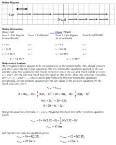
A car, initially at rest, accelerates toward the west at 2.0 m/s2. At the same time that the car starts, a truck, 350 m west of the car and moving at 16 m/s toward the east, starts to move slower, accelerating at 1.0 m/s2. The car and truck pass safely.
Motion Diagram
Motion Information
Object: Object:
| Event 1:
t1 = r1 = v1 = a12 = |
Event 2:
t2 = r2 = v2 =
|
Event 1:
t1 = r1 = v1 = a12 = |
Event 2:
t2 = r2 = v2 =
|
Mathematical Analysis
A car, initially traveling at 20 m/s to the east, accelerates toward the west at 2.0 m/s2. At the same time that the car starts, a truck, 60 m west of the car and moving at 16 m/s toward the east, starts to move faster, accelerating at 1.0 m/s2. It’s a one-lane road and both drivers are too busy texting to notice each other.
Motion Diagram
Motion Information
Object: Object:
| Event 1:
t1 = r1 = v1 = a12 = |
Event 2:
t2 = r2 = v2 =
|
Event 1:
t1 = r1 = v1 = a12 = |
Event 2:
t2 = r2 = v2 =
|
Mathematical Analysis[xi]
A helium balloon begins to rise from rest with an acceleration of 2.0 m/s2 until it reaches a height of 50 m, and then continues upward at constant speed. However, a passenger in the balloon forgot their cell phone on the ground and threatens to jump from the balloon because of separation anxiety. Therefore a second balloon is launched 5.0 s after the first and accelerates upwards at 3.0 m/s2 to reunite the passenger and his phone.
Motion Diagram Motion Information
| Object:
Event 1:
t1 = r1 = v1 = a12 =
|
Event 2:
t2 = r2 = v2 = a23 = |
Event 3:
t3 = r3 = v3 =
|
Object:
Event 1:
t1 = r1 = v1 = a12 = |
Event 2:
t2 = r2 = v2 = a23 =
|
Event 3:
t3 = r3 = v3 =
|
Mathematical Analysis[xii]
A car traveling at 16 m/s sees a truck 20 m ahead traveling at a constant speed of 12 m/s. After thinking it over for 0.80 s, the car starts to accelerate at 4.0 m/s2 in an attempt to rear-end the truck. The truck driver has paid-up insurance so doesn’t care. The car driver’s motive is unknown.
Motion Diagram
Motion Information
Object: Object:
| Event 1:
t1 = r1 = v1 = a12 = |
Event 2:
t2 = r2 = v2 = a23 = |
Event 3:
t3 = r3 = v3 =
|
Event 1:
t1 = r1 = v1 = a12 = |
Event 2:
t2 = r2 = v2 = a23 = |
Event 3:
t3 = r3 = v3 =
|
Mathematical Analysis[xiii]
A pole-vaulter lands on a cushion after a vault. Determine her acceleration as she sinks into the cushion (acushion) as a function of her velocity when she hits the cushion (vi) and the distance she sinks into the cushion (d).
Motion Diagram Motion Information
| Event 1:
t1 = r1 = v1 = a12 = Mathematical Analysis
|
Event 2:
t2 = r2 = v2 =
|
Questions
If vi = 0 m/s, what should acushion equal? Does your function agree with this observation?
If d = 0 m, what should acushion equal? Does your function agree with this observation?
What would result in a larger magnitude acceleration, hitting the cushion twice as fast or sinking one-half as far into the cushion?
The driver of an automobile suddenly sees an obstacle blocking her lane. Determine the total distance the car travels between seeing the obstacle and stopping (d) as a function of the initial velocity of the car (vi) and the magnitude of the car’s acceleration while stopping (as). Ignore the driver’s reaction time.
Motion Diagram
Motion Information
| Event 1:
t1 = r1 = v1 = a12 = |
Event 2:
t2 = r2 = v2 =
|
Mathematical Analysis
Questions
If vi = 0 m/s, what should d equal? Does your function agree with this observation?
If as = 0 m/s2, what should d equal? Does your function agree with this observation?
If the car was traveling twice as fast how much further would the car travel before stopping?
The driver of an automobile suddenly sees an obstacle blocking his lane. Determine the total distance the car travels between seeing the obstacle and stopping (d) as a function of his reaction time (tR), the initial velocity of the car (vi), and the magnitude of the car’s acceleration while stopping (as).
Motion Diagram
Motion Information
| Event 1:
t1 = r1 = v1 = a12 = |
Event 2:
t2 = r2 = v2 = a23 = |
Event 3:
t3 = r3 = v3 =
|
Mathematical Analysis
Questions
If vi = 0 m/s, what should d equal? Does your function agree with this observation?
If as = 0 m/s2, what should d equal? Does your function agree with this observation?
Does the car travel a greater distance during the reaction phase or the braking phase? Estimate necessary quantities assuming a panic stop from highway speeds.
Two automobiles are involved in a race over level ground. Both cars begin at rest. The Audi accelerates at A for T seconds and then travels at constant velocity for the rest of the race. The Buick accelerates at A/2 for 2T seconds and then travels at constant velocity for the rest of the race. Determine the distance (d) between the two cars, at the instant t = 2T, as a function of A and T.
Motion Diagram
Motion Information
Object: Object:
| Event 1:
t1 = r1 = v1 = a12 = |
Event 2:
t2 = r2 = v2 = a23 = |
Event 3:
t3 = r3 = v3 =
|
Event 1:
t1 = r1 = v1 = a12 = |
Event 2:
t2 = r2 = v2 = a23 = |
Event 3:
t3 = r3 = v3 =
|
Mathematical Analysis
Questions
If A = 0 m/s2, what should d equal? Does your function agree with this observation?
Assume the race takes longer than 2T to finish. What is the difference in speed between the two cars as they cross the finish line?
Assume the race takes longer than 2T to finish. What is the distance between the two cars as they cross the finish line?
Two automobiles are involved in a game of chicken. The two cars start from rest at opposite ends of a long, one-lane road. The Audi accelerates at A for T seconds and then travels at constant velocity. The Buick accelerates at A/2 for 2T seconds and then travels at constant velocity. Determine the elapsed time when the car’s collide (tcollide) as a function of the length of the road (d), A and T. The collision takes place after both cars have reached constant velocity.
Motion Diagram
Motion Information
Object: Object:
| Event 1:
t1 = r1 = v1 = a12 = |
Event 2:
t2 = r2 = v2 = a23 = |
Event 3:
t3 = r3 = v3 =
|
Event 1:
t1 = r1 = v1 = a12 = |
Event 2:
t2 = r2 = v2 = a23 = |
Event 3:
t3 = r3 = v3 =
|
Mathematical Analysis
Questions
If A = 0 m/s2, what should tcollide equal? Does your function agree with this observation?
If d = ∞, what should tcollide equal? Does your function agree with this observation?
What is the minimum length of road needed to guarantee the two cars collide at top speed?
[ii] t2 = 1.45 m
[iii] t3 = 3.4 s
[iv] t3 = 4.55 s
[v] r3 = 36.6 m
[vi] r3 = 3520 m
[vii] r2 = 14.9 m
[viii] r4 = 2000 m
[ix] t4 = 3.7 x 10⁵ s
[x] t2 = 14.9 s
[xi] t2 = 7.8 s
[xii] t3 = 15.7 s
[xiii] t3 = 2.87 s
Homework 1 – Model 1: 25, 31, 32, 35, 39, 45, 47, 53, 55, and 59.
Candela Citations
- University Physics I Homework Assignments. Authored by: Mary Mohr. License: CC BY-NC-SA: Attribution-NonCommercial-ShareAlike
- These two relationships are simply the definitions of velocity and acceleration rearranged. I show all the steps in the addendum to this chapter. ↵


