How Perfectly Competitive Firms Make Output Decisions
A perfectly competitive firm has only one major decision to make—namely, what quantity to produce. To understand why this is so, consider a different way of writing out the basic definition of profit:
| Profit | = Total Revenue – Total Cost |
| = (Price)(Quantity Produced) – (Average Cost)(Quantity Produced) |
Since a perfectly competitive firm must accept the price for its output as determined by the product’s market demand and supply, it cannot choose the price it charges. This is already determined in the profit equation, and so the perfectly competitive firm can sell any number of units at exactly the same price. It implies that the firm faces a perfectly elastic demand curve for its product: buyers are willing to buy any number of units of output from the firm at the market price. When the perfectly competitive firm chooses what quantity to produce, then this quantity—along with the prices prevailing in the market for output and inputs—will determine the firm’s total revenue, total costs, and ultimately, level of profits.
DETERMINING THE HIGHEST PROFIT BY COMPARING TOTAL REVENUE AND TOTAL COST
A perfectly competitive firm can sell as large a quantity as it wishes, as long as it accepts the prevailing market price. Total revenue is going to increase as the firm sells more, depending on the price of the product and the number of units sold. If you increase the number of units sold at a given price, then total revenue will increase. If the price of the product increases for every unit sold, then total revenue also increases. As an example of how a perfectly competitive firm decides what quantity to produce, consider the case of a small farmer who produces raspberries and sells them frozen for $4 per pack. Sales of one pack of raspberries will bring in $4, two packs will be $8, three packs will be $12, and so on. If, for example, the price of frozen raspberries doubles to $8 per pack, then sales of one pack of raspberries will be $8, two packs will be $16, three packs will be $24, and so on.
Total revenue and total costs for the raspberry farm, broken down into fixed and variable costs, are shown in Table 8.1 and also appear in Figure 8.2. The horizontal axis shows the quantity of frozen raspberries produced in packs; the vertical axis shows both total revenue and total costs, measured in dollars. The total cost curve intersects with the vertical axis at a value that shows the level of fixed costs, and then slopes upward. All these cost curves follow the same characteristics as the curves covered in the Cost and Industry Structure module.

Figure 8.2. Total Cost and Total Revenue at the Raspberry Farm. Total revenue for a perfectly competitive firm is a straight line sloping up. The slope is equal to the price of the good. Total cost also slopes up, but with some curvature. At higher levels of output, total cost begins to slope upward more steeply because of diminishing marginal returns. The maximum profit will occur at the quantity where the gap of total revenue over total cost is largest.
Table 8.1 Total Cost and Total Revenue at the Raspberry Farm
| Quantity
(Q) |
Total Cost
(TC) |
Fixed Cost
(FC) |
Variable Cost
(VC) |
Total Revenue
(TR) |
Profit |
|---|---|---|---|---|---|
| 0 | $62 | $62 | – | $0 | −$62 |
| 10 | $90 | $62 | $28 | $40 | −$50 |
| 20 | $110 | $62 | $48 | $80 | −$30 |
| 30 | $126 | $62 | $64 | $120 | −$6 |
| 40 | $144 | $62 | $82 | $160 | $16 |
| 50 | $166 | $62 | $104 | $200 | $34 |
| 60 | $192 | $62 | $130 | $240 | $48 |
| 70 | $224 | $62 | $162 | $280 | $56 |
| 80 | $264 | $62 | $202 | $320 | $56 |
| 90 | $324 | $62 | $262 | $360 | $36 |
| 100 | $404 | $62 | $342 | $400 | −$4 |
Based on its total revenue and total cost curves, a perfectly competitive firm like the raspberry farm can calculate the quantity of output that will provide the highest level of profit. At any given quantity, total revenue minus total cost will equal profit. One way to determine the most profitable quantity to produce is to see at what quantity total revenue exceeds total cost by the largest amount. On Figure 8.2, the vertical gap between total revenue and total cost represents either profit (if total revenues are greater that total costs at a certain quantity) or losses (if total costs are greater that total revenues at a certain quantity). In this example, total costs will exceed total revenues at output levels from 0 to 40, and so over this range of output, the firm will be making losses. At output levels from 50 to 80, total revenues exceed total costs, so the firm is earning profits. But then at an output of 90 or 100, total costs again exceed total revenues and the firm is making losses. Total profits appear in the final column of Table 8.1. The highest total profits in the table, as in the figure that is based on the table values, occur at an output of 70–80, when profits will be $56.
A higher price would mean that total revenue would be higher for every quantity sold. A lower price would mean that total revenue would be lower for every quantity sold. What happens if the price drops low enough so that the total revenue line is completely below the total cost curve; that is, at every level of output, total costs are higher than total revenues? In this instance, the best the firm can do is to suffer losses. But a profit-maximizing firm will prefer the quantity of output where total revenues come closest to total costs and thus where the losses are smallest.
(Later we will see that sometimes it will make sense for the firm to shutdown, rather than stay in operation producing output.)
Watch the following video to learn more about the point of profit maximization.
COMPARING MARGINAL REVENUE AND MARGINAL COSTS
Firms often do not have the necessary data they need to draw a complete total cost curve for all levels of production. They cannot be sure of what total costs would look like if they, say, doubled production or cut production in half, because they have not tried it. Instead, firms experiment. They produce a slightly greater or lower quantity and observe how profits are affected. In economic terms, this practical approach to maximizing profits means looking at how changes in production affect marginal revenue and marginal cost.
Figure 8.3 presents the marginal revenue and marginal cost curves based on the total revenue and total cost in Table 8.1. The marginal revenue curve shows the additional revenue gained from selling one more unit. As mentioned before, a firm in perfect competition faces a perfectly elastic demand curve for its product—that is, the firm’s demand curve is a horizontal line drawn at the market price level. This also means that the firm’s marginal revenue curve is the same as the firm’s demand curve: Every time a consumer demands one more unit, the firm sells one more unit and revenue goes up by exactly the same amount equal to the market price. In this example, every time a pack of frozen raspberries is sold, the firm’s revenue increases by $4. Table 8.2 shows an example of this. This condition only holds for price taking firms in perfect competition where: marginal revenue = price.
The formula for marginal revenue is:
[latex]\text{marginal revenue}=\frac{\text{change in total revenue}}{\text{change in quantity}}[/latex]
Table 8.2 Marginal Revenue
| Price | Quantity | Total Revenue | Marginal Revenue |
|---|---|---|---|
| $4 | 1 | $4 | – |
| $4 | 2 | $8 | $4 |
| $4 | 3 | $12 | $4 |
| $4 | 4 | $16 | $4 |
Notice that marginal revenue does not change as the firm produces more output. That is because the price is determined by supply and demand and does not change as the farmer produces more (keeping in mind that, due to the relative small size of each firm, increasing their supply has no impact on the total market supply where price is determined).
Since a perfectly competitive firm is a price taker, it can sell whatever quantity it wishes at the market-determined price. Marginal cost, the cost per additional unit sold, is calculated by dividing the change in total cost by the change in quantity. The formula for marginal cost is:
[latex]\text{marginal cost}=\frac{\text{change in total cost}}{\text{change in quantity}}[/latex]
Ordinarily, marginal cost changes as the firm produces a greater quantity.
In the raspberry farm example, shown in Figure 8.3, Figure 8.4 and Table 8.3, marginal cost at first declines as production increases from 10 to 20 to 30 packs of raspberries—which represents the area of increasing marginal returns that is not uncommon at low levels of production. But then marginal costs start to increase, displaying the typical pattern of diminishing marginal returns. If the firm is producing at a quantity where MR > MC, like 40 or 50 packs of raspberries, then it can increase profit by increasing output because the marginal revenue is exceeding the marginal cost. If the firm is producing at a quantity where MC > MR, like 90 or 100 packs, then it can increase profit by reducing output because the reductions in marginal cost will exceed the reductions in marginal revenue. The firm’s profit-maximizing choice of output will occur where MR = MC (or at a choice close to that point). You will notice that what occurs on the production side is exemplified on the cost side. This is referred to as duality.

Figure 8.3. Marginal Revenues and Marginal Costs at the Raspberry Farm: Individual Farmer. For a perfectly competitive firm, the marginal revenue (MR) curve is a horizontal straight line because it is equal to the price of the good, which is determined by the market, shown in Figure 8.4. The marginal cost (MC) curve is sometimes first downward-sloping, if there is a region of increasing marginal returns at low levels of output, but is eventually upward-sloping at higher levels of output as diminishing marginal returns kick in.
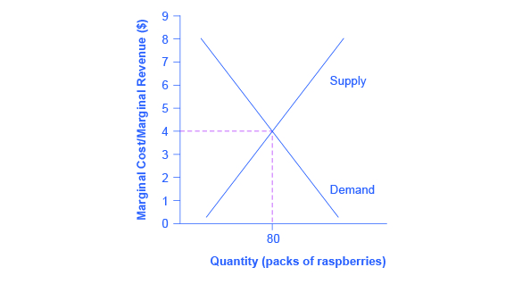
Figure 8.4. Marginal Revenues and Marginal Costs at the Raspberry Farm: Raspberry Market. The equilibrium price of raspberries is determined through the interaction of market supply and market demand at $4.00.
Table 8.3 Marginal Revenues and Marginal Costs at the Raspberry Farm
| Quantity | Total Cost | Fixed Cost | Variable Cost | Marginal Cost | Total Revenue | Marginal Revenue |
|---|---|---|---|---|---|---|
| 0 | $62 | $62 | – | – | – | – |
| 10 | $90 | $62 | $28 | $2.80 | $40 | $4.00 |
| 20 | $110 | $62 | $48 | $2.00 | $80 | $4.00 |
| 30 | $126 | $62 | $64 | $1.60 | $120 | $4.00 |
| 40 | $144 | $62 | $82 | $1.80 | $160 | $4.00 |
| 50 | $166 | $62 | $104 | $2.20 | $200 | $4.00 |
| 60 | $192 | $62 | $130 | $2.60 | $240 | $4.00 |
| 70 | $224 | $62 | $162 | $3.20 | $280 | $4.00 |
| 80 | $264 | $62 | $202 | $4.00 | $320 | $4.00 |
| 90 | $324 | $62 | $262 | $6.00 | $360 | $4.00 |
| 100 | $404 | $62 | $342 | $8.00 | $400 | $4.00 |
In this example, the marginal revenue and marginal cost curves cross at a price of $4 and a quantity of 80 produced. If the farmer started out producing at a level of 60, and then experimented with increasing production to 70, marginal revenues from the increase in production would exceed marginal costs—and so profits would rise. The farmer has an incentive to keep producing. From a level of 70 to 80, marginal cost and marginal revenue are equal so profit doesn’t change. If the farmer then experimented further with increasing production from 80 to 90, he would find that marginal costs from the increase in production are greater than marginal revenues, and so profits would decline.
The profit-maximizing choice for a perfectly competitive firm will occur where marginal revenue is equal to marginal cost—that is, where MR = MC. A profit-seeking firm should keep expanding production as long as MR > MC. But at the level of output where MR = MC, the firm should recognize that it has achieved the highest possible level of economic profits. (In the example above, the profit maximizing output level is between 70 and 80 units of output, but the firm will not know they’ve maximized profit until they reach 80, where MR = MC.) Expanding production into the zone where MR < MC will only reduce economic profits. Because the marginal revenue received by a perfectly competitive firm is equal to the price P, so that P = MR, the profit-maximizing rule for a perfectly competitive firm can also be written as a recommendation to produce at the quantity where P = MC.
Self Check: Costs and Revenues in Competitive Markets
Answer the question(s) below to see how well you understand the topics covered in the previous section. This short quiz does not count toward your grade in the class, and you can retake it an unlimited number of times.
You’ll have more success on the Self Check if you’ve completed the Reading in this section.
Use this quiz to check your understanding and decide whether to (1) study the previous section further or (2) move on to the next section.
Candela Citations
- Principles of Microeconomics Chapter 8.2. Authored by: OpenStax College. Located at: http://cnx.org/contents/6i8iXmBj@10.31:9ACVqdAi@13/How-Perfectly-Competitive-Firm. License: CC BY: Attribution. License Terms: Download for free at http://cnx.org/content/col11627/latest
- Perfect competition: Point of profit maximisation. Authored by: lostmy1. Provided by: University of South Africa. Located at: https://youtu.be/RTbqy8vSzFs?list=PL616B7E47EF9203CC. License: CC BY: Attribution