The purpose of this assignment:
1. Enter and change labels
2. Enter and change values
3. Use the AutoSum Key
Preparation: (Review these terms and readings)
- Read Building a Spreadsheet, pages 1 and 2
- Understand terms label, value, Cell Referencing
New terms: (Terms are bolded in the steps)
- AutoSum Key (#6 & 7)
- Shortcut to AutoFill (#8)
Helpful Hints:
Narrative:
This first assignment will help you understand how to set up a typical spreadsheet. Following each assignment is a rubric explaining the points values for components of the assignment. (THIS ASSIGNMENT IS WORTH 5 POINTS. THE RUBRIC IS ON PAGE 3.)
Test Score Assignment
- Open a blank worksheet and SAVE it with the name: Test Scores
- Below is a diagram of a table. The words “column” and “row” are diagramed here for clarification only. On your spreadsheet, you will find only letters and numbers. Remember columns are horizontal and rows are vertical in a spreadsheet. Column letters are referenced before Row numbers. Go to step 3.

- Insert Labels in the Test Scores spreadsheet cells as indicated.
- Type Name in cell A4 (Column A, Row 4)
- Type Test 1 in cell B4 (Column B, Row 4)
- Type Test 2 in cell C4 (Column C, Row 4)
- Type Test 3 in cell D4 (Column D, Row 4)
- Type Total Points in cell E4 (Column E, Row 4)
- Insert the names and test scores data in each of the cells as indicated. Do not put any information in the “Total Points” column at this time. Remember if all the information typed in a cell, widen the cell. ([HINT: SEE BASIC DEFINITIONS: LABELS #3. ON THE “BUILDING A SPREADSHEET” INFORMATION SHEET]
- Click your mouse pointer in cell E5. This makes the cell “active.” You should be under “Total Points” for Susi Q.
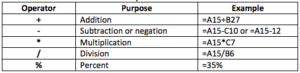
- Click on the AutoSum key. [HINT: SEE BASIC DEFINITION: AUTOSUM #1]
- Press the AutoSum key found by clicking HOME tab, finding Editing Group, and clicking on AutoSum icon. The spreadsheet programs knows that from this position, values will be added horizontally. The AutoSum key placed a dotted line around the entire row. The formula in cell E5 that displays is also mirrored in the formula bar (fx) just under the ribbon. The formula that automatically shows up is =SUM(A5:D5). Press ENTER. A total appears of 235.
- Once the formula has been placed in E5, we could use the AutoSum key again for the next row. = However, an excellent shortcut is called Auto Fill. [Directions: CLICK IN E5 WHERE THE ORIGINAL FORMULA IS. IN THE LOWER RIGHT CORNER OF CELL E5 THERE IS A TINY SQUARE. PLACE YOUR MOUSE CURSOR ON THAT TINY SQUARE. IT SHOULD TURN INTO A BLACK PLUS SIGN. WHEN IT DOES, HOLD DOWN YOUR LEFT MOUSE BUTTON AND DRAG THE FORMULA DOWN TO E7. RELEASE THE MOUSE. THE FORMULA HAS BEEN INSERTED INTO EACH OF THE OTHER CELLS.]
- You will note that on each row, the Row Number changed automatically. For example: Celia’s sum is =SUM(A6:D6); Jumping Bean is =SUM(A7:D7).
- Put your name in cell A1 and save this table to your storage device once again as Test Scores.
- If you are submitting your work through Blackboard, follow the instructions given to you for this assignment on the Blackboard screen.
- If you are in a classroom, print this assignment out for your instructor.
Check the rubric below to be sure you have completed all the tasks. 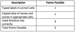
Candela Citations
CC licensed content, Original
- Test Scores Assignment. Authored by: Fran Wells. License: CC BY: Attribution