Learning Outcomes
- Model exponential growth and decay
One of the main topics covered in the Exponential and Logarithmic Functions section is graphing exponential functions. The ability to identify whether an exponential function represents exponential growth or decay, which is reviewed here, is an important aspect of determining the shape of its graph.
Identify Exponential Growth and Decay
In real-world applications, we need to model the behavior of a function. In mathematical modeling, we choose a familiar general function with properties that suggest that it will model the real-world phenomenon we wish to analyze. In the case of rapid growth (or decay), we may choose to model the given scenario using the following function:
[latex]y={A}_{0}{b}^{x}[/latex]
where [latex]{A}_{0}[/latex] is equal to the value at [latex]x=0[/latex], [latex]b[/latex] is the base, and [latex]x[/latex] is the exponent. Note that the variable is in the exponent which makes the function exponential.
When [latex]b>0[/latex], the exponential function represents exponential growth. Common applications of exponential growth include doubling time, the time it takes for a quantity to double. Such phenomena as wildlife populations, financial investments, biological samples, and natural resources may exhibit growth based on a doubling time.
When [latex]b<0[/latex], the exponential function represents exponential decay. One common application of exponential decay includes calculating half-life, or the time it takes for a substance to exponentially decay to half of its original quantity. We use half-life in applications involving radioactive isotopes.
In our choice of a function to serve as a mathematical model, we often use data points gathered by careful observation and measurement to construct points on a graph and hope we can recognize the shape of the graph. Exponential growth and decay graphs have a distinctive shape, as we can see in the graphs below. It is important to remember that, although parts of each of the two graphs seem to lie on the x-axis, they are really a tiny distance above the x-axis.
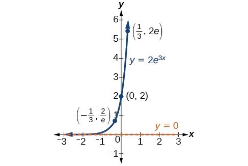
A graph showing exponential growth. The equation is [latex]y=2{e}^{3x}[/latex].
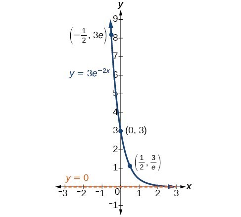
A graph showing exponential decay. The equation is [latex]y=3{e}^{-2x}[/latex].
A General Note: Characteristics of the Exponential Function [latex]y=A_{0}b^{x}[/latex]
An exponential function of the form [latex]y={A}_{0}{b}^{x}[/latex] has the following characteristics:
- one-to-one function
- horizontal asymptote: y = 0
- domain: [latex]\left(-\infty , \infty \right)[/latex]
- range: [latex]\left(0,\infty \right)[/latex]
- x intercept: none
- y-intercept: [latex]\left(0,{A}_{0}\right)[/latex]
- increasing if b > 0
- decreasing if b < 0
An exponential function models exponential growth when [latex]b > 0[/latex] and exponential decay when [latex]b < 0[/latex].
Try It
Try It
Candela Citations
- Modification and Revision. Provided by: Lumen Learning. License: CC BY: Attribution
- College Algebra Corequisite. Provided by: Lumen Learning. Located at: https://courses.lumenlearning.com/waymakercollegealgebracorequisite/. License: CC BY: Attribution
- Precalculus. Provided by: Lumen Learning. Located at: https://courses.lumenlearning.com/precalculus/. License: CC BY: Attribution
