Learning Outcomes
- Describe the steps of Newton’s method
- Explain what an iterative process means
- Recognize when Newton’s method does not work
Describing Newton’s Method
Consider the task of finding the solutions of [latex]f(x)=0[/latex]. If [latex]f[/latex] is the first-degree polynomial [latex]f(x)=ax+b[/latex], then the solution of [latex]f(x)=0[/latex] is given by the formula [latex]x=-\frac{b}{a}[/latex]. If [latex]f[/latex] is the second-degree polynomial [latex]f(x)=ax^2+bx+c[/latex], the solutions of [latex]f(x)=0[/latex] can be found by using the quadratic formula. However, for polynomials of degree 3 or more, finding roots of [latex]f[/latex] becomes more complicated. Although formulas exist for third- and fourth-degree polynomials, they are quite complicated. Also, if [latex]f[/latex] is a polynomial of degree 5 or greater, it is known that no such formulas exist. For example, consider the function
No formula exists that allows us to find the solutions of [latex]f(x)=0[/latex]. Similar difficulties exist for nonpolynomial functions. For example, consider the task of finding solutions of [latex]\tan (x)-x=0[/latex]. No simple formula exists for the solutions of this equation. In cases such as these, we can use Newton’s method to approximate the roots.
Newton’s method makes use of the following idea to approximate the solutions of [latex]f(x)=0[/latex]. By sketching a graph of [latex]f[/latex], we can estimate a root of [latex]f(x)=0[/latex]. Let’s call this estimate [latex]x_0[/latex]. We then draw the tangent line to [latex]f[/latex] at [latex]x_0[/latex]. If [latex]f^{\prime}(x_0)\ne 0[/latex], this tangent line intersects the [latex]x[/latex]-axis at some point [latex](x_1,0)[/latex]. Now let [latex]x_1[/latex] be the next approximation to the actual root. Typically, [latex]x_1[/latex] is closer than [latex]x_0[/latex] to an actual root. Next we draw the tangent line to [latex]f[/latex] at [latex]x_1[/latex]. If [latex]f^{\prime}(x_1)\ne 0[/latex], this tangent line also intersects the [latex]x[/latex]-axis, producing another approximation, [latex]x_2[/latex]. We continue in this way, deriving a list of approximations: [latex]x_0, x_1, x_2, \cdots[/latex]. Typically, the numbers [latex]x_0,x_1,x_2, \cdots[/latex] quickly approach an actual root [latex]x*[/latex], as shown in the following figure.
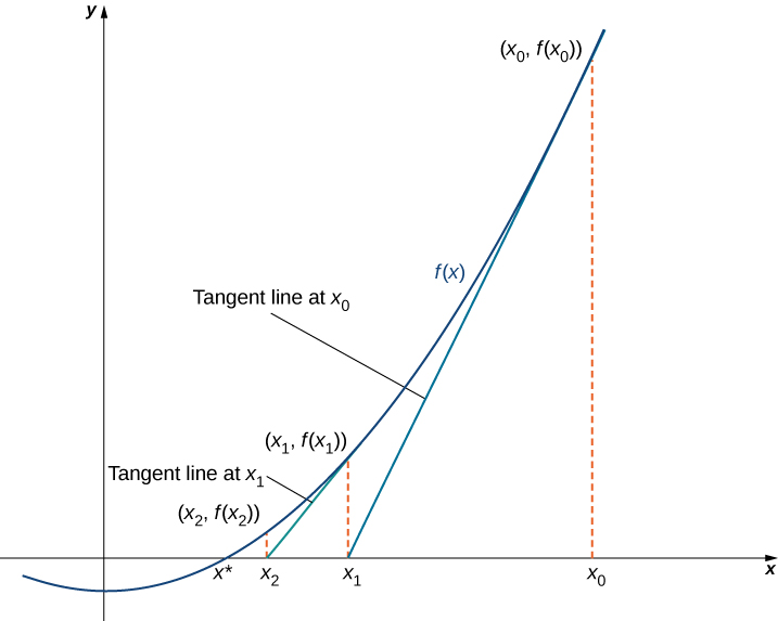
Figure 1. The approximations [latex]x_0,x_1,x_2, \cdots[/latex] approach the actual root [latex]x*[/latex]. The approximations are derived by looking at tangent lines to the graph of [latex]f[/latex].
Now let’s look at how to calculate the approximations [latex]x_0,x_1,x_2, \cdots[/latex]. If [latex]x_0[/latex] is our first approximation, the approximation [latex]x_1[/latex] is defined by letting [latex](x_1,0)[/latex] be the [latex]x[/latex]-intercept of the tangent line to [latex]f[/latex] at [latex]x_0[/latex]. The equation of this tangent line is given by
Solving this equation for [latex]x_1[/latex], we conclude that
Similarly, the point [latex](x_2,0)[/latex] is the [latex]x[/latex]-intercept of the tangent line to [latex]f[/latex] at [latex]x_1[/latex]. Therefore, [latex]x_2[/latex] satisfies the equation
In general, for [latex]n>0, \, x_n[/latex] satisfies
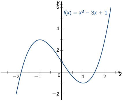
Next we see how to make use of this technique to approximate the root of the polynomial [latex]f(x)=x^3-3x+1[/latex].
Example: Finding a Root of a Polynomial
Use Newton’s method to approximate a root of [latex]f(x)=x^3-3x+1[/latex] in the interval [latex][1,2][/latex]. Let [latex]x_0=2[/latex] and find [latex]x_1,x_2,x_3,x_4[/latex], and [latex]x_5[/latex].
Watch the following video to see the worked solution to Example: Finding a Root of a Polynomial.
Try It
Letting [latex]x_0=0[/latex], use Newton’s method to approximate the root of [latex]f(x)=x^3-3x+1[/latex] over the interval [latex][0,1][/latex] by calculating [latex]x_1[/latex] and [latex]x_2[/latex].
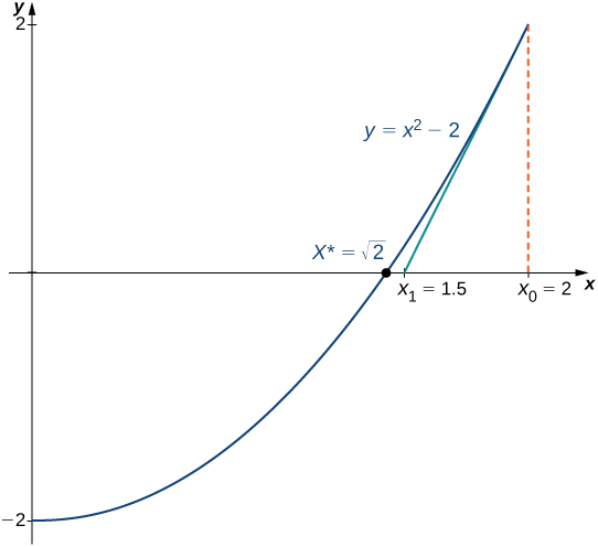
Newton’s method can also be used to approximate square roots. Here we show how to approximate [latex]\sqrt{2}[/latex]. This method can be modified to approximate the square root of any positive number.
example: Finding a Square Root
Use Newton’s method to approximate [latex]\sqrt{2}[/latex] (Figure 3). Let [latex]f(x)=x^2-2[/latex], let [latex]x_0=2[/latex], and calculate [latex]x_1,x_2,x_3,x_4,x_5[/latex]. (We note that since [latex]f(x)=x^2-2[/latex] has a zero at [latex]\sqrt{2}[/latex], the initial value [latex]x_0=2[/latex] is a reasonable choice to approximate [latex]\sqrt{2}[/latex].)
Try It
Use Newton’s method to approximate [latex]\sqrt{3}[/latex] by letting [latex]f(x)=x^2-3[/latex] and [latex]x_0=3[/latex]. Find [latex]x_1[/latex] and [latex]x_2[/latex].
Try It
When using Newton’s method, each approximation after the initial guess is defined in terms of the previous approximation by using the same formula. In particular, by defining the function [latex]F(x)=x-\left[\frac{f(x)}{f^{\prime}(x)}\right][/latex], we can rewrite the equation for[latex]x_n[/latex] as [latex]x_n=F(x_{n-1})[/latex]. This type of process, where each [latex]x_n[/latex] is defined in terms of [latex]x_{n-1}[/latex] by repeating the same function, is an example of an iterative process. Shortly, we examine other iterative processes. First, let’s look at the reasons why Newton’s method could fail to find a root.
Failures of Newton’s Method
Typically, Newton’s method is used to find roots fairly quickly. However, things can go wrong. Some reasons why Newton’s method might fail include the following:
- At one of the approximations [latex]x_n[/latex], the derivative [latex]f^{\prime}[/latex] is zero at [latex]x_n[/latex], but [latex]f(x_n) \ne 0[/latex]. As a result, the tangent line of [latex]f[/latex] at [latex]x_n[/latex] does not intersect the [latex]x[/latex]-axis. Therefore, we cannot continue the iterative process.
- The approximations [latex]x_0,x_1,x_2, \cdots[/latex] may approach a different root. If the function [latex]f[/latex] has more than one root, it is possible that our approximations do not approach the one for which we are looking, but approach a different root (see Figure 4). This event most often occurs when we do not choose the approximation [latex]x_0[/latex] close enough to the desired root.
- The approximations may fail to approach a root entirely. In the example below, we provide an example of a function and an initial guess [latex]x_0[/latex] such that the successive approximations never approach a root because the successive approximations continue to alternate back and forth between two values.
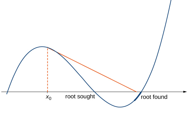
Figure 4. If the initial guess [latex]x_0[/latex] is too far from the root sought, it may lead to approximations that approach a different root.
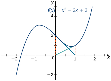
example: When Newton’s Method Fails
Consider the function [latex]f(x)=x^3-2x+2[/latex]. Let [latex]x_0=0[/latex]. Show that the sequence [latex]x_1,x_2, \cdots[/latex] fails to approach a root of [latex]f[/latex].
Watch the following video to see the worked solution to Example: When Newton’s Method Fails.
Try It
For [latex]f(x)=x^3-2x+2[/latex], let [latex]x_0=-1.5[/latex] and find [latex]x_1[/latex] and [latex]x_2[/latex].
From the example above, we see that Newton’s method does not always work. However, when it does work, the sequence of approximations approaches the root very quickly. Discussions of how quickly the sequence of approximations approach a root found using Newton’s method are included in texts on numerical analysis.
Candela Citations
- 4.9 Newton's Method. Authored by: Ryan Melton. License: CC BY: Attribution
- Calculus Volume 1. Authored by: Gilbert Strang, Edwin (Jed) Herman. Provided by: OpenStax. Located at: https://openstax.org/details/books/calculus-volume-1. License: CC BY-NC-SA: Attribution-NonCommercial-ShareAlike. License Terms: Access for free at https://openstax.org/books/calculus-volume-1/pages/1-introduction
