Learning Outcomes
- Find the center of mass of objects distributed along a line.
- Locate the center of mass of a thin plate.
- Use symmetry to help locate the centroid of a thin plate.
Center of Mass and Moments
Let’s begin by looking at the center of mass in a one-dimensional context. Consider a long, thin wire or rod of negligible mass resting on a fulcrum, as shown in Figure 1(a). Now suppose we place objects having masses [latex]{m}_{1}[/latex] and [latex]{m}_{2}[/latex] at distances [latex]{d}_{1}[/latex] and [latex]{d}_{2}[/latex] from the fulcrum, respectively, as shown in Figure 1(b).
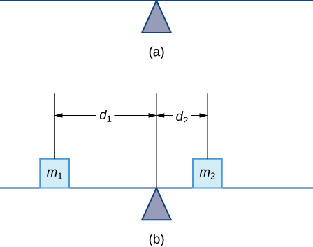
Figure 1. (a) A thin rod rests on a fulcrum. (b) Masses are placed on the rod.
The most common real-life example of a system like this is a playground seesaw, or teeter-totter, with children of different weights sitting at different distances from the center. On a seesaw, if one child sits at each end, the heavier child sinks down and the lighter child is lifted into the air. If the heavier child slides in toward the center, though, the seesaw balances. Applying this concept to the masses on the rod, we note that the masses balance each other if and only if [latex]{m}_{1}{d}_{1}={m}_{2}{d}_{2}.[/latex]
In the seesaw example, we balanced the system by moving the masses (children) with respect to the fulcrum. However, we are really interested in systems in which the masses are not allowed to move, and instead we balance the system by moving the fulcrum. Suppose we have two point masses, [latex]{m}_{1}[/latex] and [latex]{m}_{2},[/latex] located on a number line at points [latex]{x}_{1}[/latex] and [latex]{x}_{2},[/latex] respectively (Figure 2). The center of mass, [latex]\overline{x},[/latex] is the point where the fulcrum should be placed to make the system balance.
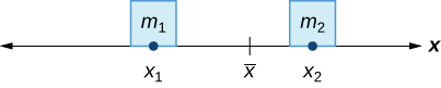
Figure 2. The center of mass [latex]\overline{x}[/latex] is the balance point of the system.
Thus, we have
The expression in the numerator, [latex]{m}_{1}{x}_{1}+{m}_{2}{x}_{2},[/latex] is called the first moment of the system with respect to the origin. If the context is clear, we often drop the word first and just refer to this expression as the moment of the system. The expression in the denominator, [latex]{m}_{1}+{m}_{2},[/latex] is the total mass of the system. Thus, the center of mass of the system is the point at which the total mass of the system could be concentrated without changing the moment.
This idea is not limited just to two point masses. In general, if [latex]n[/latex] masses, [latex]{m}_{1},{m}_{2}\text{,…},{m}_{n},[/latex] are placed on a number line at points [latex]{x}_{1},{x}_{2}\text{,…},{x}_{n},[/latex] respectively, then the center of mass of the system is given by
Center of Mass of Objects on a Line
Let [latex]{m}_{1},{m}_{2}\text{,…},{m}_{n}[/latex] be point masses placed on a number line at points [latex]{x}_{1},{x}_{2}\text{,…},{x}_{n},[/latex] respectively, and let [latex]m=\underset{i=1}{\overset{n}{\text{∑}}}{m}_{i}[/latex] denote the total mass of the system. Then, the moment of the system with respect to the origin is given by
and the center of mass of the system is given by
We apply this theorem in the following example.
Example: Finding the Center of Mass of Objects along a Line
Suppose four point masses are placed on a number line as follows:
Find the moment of the system with respect to the origin and find the center of mass of the system.
Try It
Suppose four point masses are placed on a number line as follows:
Find the moment of the system with respect to the origin and find the center of mass of the system.
We can generalize this concept to find the center of mass of a system of point masses in a plane. Let [latex]{m}_{1}[/latex] be a point mass located at point [latex]({x}_{1},{y}_{1})[/latex] in the plane. Then the moment [latex]{M}_{x}[/latex] of the mass with respect to the [latex]x[/latex]-axis is given by [latex]{M}_{x}={m}_{1}{y}_{1}.[/latex] Similarly, the moment [latex]{M}_{y}[/latex] with respect to the [latex]y[/latex]-axis is given by [latex]{M}_{y}={m}_{1}{x}_{1}.[/latex] Notice that the [latex]x[/latex]-coordinate of the point is used to calculate the moment with respect to the [latex]y[/latex]-axis, and vice versa. The reason is that the [latex]x[/latex]-coordinate gives the distance from the point mass to the [latex]y[/latex]-axis, and the [latex]y[/latex]-coordinate gives the distance to the [latex]x[/latex]-axis (see the following figure).
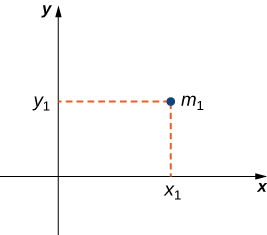
Figure 3. Point mass [latex]{m}_{1}[/latex] is located at point [latex]({x}_{1},{y}_{1})[/latex] in the plane.
If we have several point masses in the xy-plane, we can use the moments with respect to the [latex]x[/latex]– and [latex]y[/latex]-axes to calculate the [latex]x[/latex]– and [latex]y[/latex]-coordinates of the center of mass of the system.
Center of Mass of Objects in a Plane
Let [latex]{m}_{1},{m}_{2}\text{,…},{m}_{n}[/latex] be point masses located in the xy-plane at points [latex]({x}_{1},{y}_{1}),({x}_{2},{y}_{2})\text{,…},({x}_{n},{y}_{n}),[/latex] respectively, and let [latex]m=\underset{i=1}{\overset{n}{\text{∑}}}{m}_{i}[/latex] denote the total mass of the system. Then the moments [latex]{M}_{x}[/latex] and [latex]{M}_{y}[/latex] of the system with respect to the [latex]x[/latex]– and [latex]y[/latex]-axes, respectively, are given by
Also, the coordinates of the center of mass [latex](\overline{x},\overline{y})[/latex] of the system are
The next example demonstrates how to apply this theorem.
Example: Finding the Center of Mass of Objects in a Plane
Suppose three point masses are placed in the xy-plane as follows (assume coordinates are given in meters):
Find the center of mass of the system.
Try It
Suppose three point masses are placed on a number line as follows (assume coordinates are given in meters):
Find the center of mass of the system.
Watch the following video to see the worked solution to the above Try It.
Center of Mass of Thin Plates
So far we have looked at systems of point masses on a line and in a plane. Now, instead of having the mass of a system concentrated at discrete points, we want to look at systems in which the mass of the system is distributed continuously across a thin sheet of material. For our purposes, we assume the sheet is thin enough that it can be treated as if it is two-dimensional. Such a sheet is called a lamina. Next we develop techniques to find the center of mass of a lamina. In this section, we also assume the density of the lamina is constant.
Laminas are often represented by a two-dimensional region in a plane. The geometric center of such a region is called its centroid. Since we have assumed the density of the lamina is constant, the center of mass of the lamina depends only on the shape of the corresponding region in the plane; it does not depend on the density. In this case, the center of mass of the lamina corresponds to the centroid of the delineated region in the plane. As with systems of point masses, we need to find the total mass of the lamina, as well as the moments of the lamina with respect to the [latex]x[/latex]– and [latex]y[/latex]-axes.
We first consider a lamina in the shape of a rectangle. Recall that the center of mass of a lamina is the point where the lamina balances. For a rectangle, that point is both the horizontal and vertical center of the rectangle. Based on this understanding, it is clear that the center of mass of a rectangular lamina is the point where the diagonals intersect, which is a result of the symmetry principle, and it is stated here without proof.
The Symmetry Principle
If a region R is symmetric about a line [latex]l[/latex], then the centroid of R lies on [latex]l[/latex].
Let’s turn to more general laminas. Suppose we have a lamina bounded above by the graph of a continuous function [latex]f(x),[/latex] below by the [latex]x[/latex]-axis, and on the left and right by the lines [latex]x=a[/latex] and [latex]x=b,[/latex] respectively, as shown in the following figure.
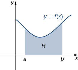
Figure 4. A region in the plane representing a lamina.
As with systems of point masses, to find the center of mass of the lamina, we need to find the total mass of the lamina, as well as the moments of the lamina with respect to the [latex]x[/latex]– and [latex]y[/latex]-axes. As we have done many times before, we approximate these quantities by partitioning the interval [latex]\left[a,b\right][/latex] and constructing rectangles.
For [latex]i=0,1,2\text{,…},n,[/latex] let [latex]P=\left\{{x}_{i}\right\}[/latex] be a regular partition of [latex]\left[a,b\right].[/latex] Recall that we can choose any point within the interval [latex]\left[{x}_{i-1},{x}_{i}\right][/latex] as our [latex]{x}_{i}^{*}.[/latex] In this case, we want [latex]{x}_{i}^{*}[/latex] to be the [latex]x[/latex]-coordinate of the centroid of our rectangles. Thus, for [latex]i=1,2\text{,…},n,[/latex] we select [latex]{x}_{i}^{*}\in \left[{x}_{i-1},{x}_{i}\right][/latex] such that [latex]{x}_{i}^{*}[/latex] is the midpoint of the interval. That is, [latex]{x}_{i}^{*}=({x}_{i-1}+{x}_{i})\text{/}2.[/latex] Now, for [latex]i=1,2\text{,…},n,[/latex] construct a rectangle of height [latex]f({x}_{i}^{*})[/latex] on [latex]\left[{x}_{i-1},{x}_{i}\right].[/latex] The center of mass of this rectangle is [latex]({x}_{i}^{*},(f({x}_{i}^{*}))\text{/}2),[/latex] as shown in the following figure.
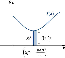
Figure 5. A representative rectangle of the lamina.
Next, we need to find the total mass of the rectangle. Let [latex]\rho[/latex] represent the density of the lamina (note that [latex]\rho[/latex] is a constant). In this case, [latex]\rho[/latex] is expressed in terms of mass per unit area. Thus, to find the total mass of the rectangle, we multiply the area of the rectangle by [latex]\rho .[/latex] Then, the mass of the rectangle is given by [latex]\rho f({x}_{i}^{*})\text{Δ}x.[/latex]
To get the approximate mass of the lamina, we add the masses of all the rectangles to get
This is a Riemann sum. Taking the limit as [latex]n\to \infty[/latex] gives the exact mass of the lamina:
Next, we calculate the moment of the lamina with respect to the [latex]x[/latex]-axis. Returning to the representative rectangle, recall its center of mass is [latex]({x}_{i}^{*},(f({x}_{i}^{*}))\text{/}2).[/latex] Recall also that treating the rectangle as if it is a point mass located at the center of mass does not change the moment. Thus, the moment of the rectangle with respect to the [latex]x[/latex]-axis is given by the mass of the rectangle, [latex]\rho f({x}_{i}^{*})\text{Δ}x,[/latex] multiplied by the distance from the center of mass to the [latex]x[/latex]-axis: [latex](f({x}_{i}^{*}))\text{/}2.[/latex] Therefore, the moment with respect to the [latex]x[/latex]-axis of the rectangle is [latex]\rho ({\left[f({x}_{i}^{*})\right]}^{2}\text{/}2)\text{Δ}x.[/latex] Adding the moments of the rectangles and taking the limit of the resulting Riemann sum, we see that the moment of the lamina with respect to the [latex]x[/latex]-axis is
We derive the moment with respect to the [latex]y[/latex]-axis similarly, noting that the distance from the center of mass of the rectangle to the [latex]y[/latex]-axis is [latex]{x}_{i}^{*}.[/latex] Then the moment of the lamina with respect to the [latex]y[/latex]-axis is given by
We find the coordinates of the center of mass by dividing the moments by the total mass to give [latex]\overline{x}={M}_{y}\text{/}m\text{ and }\overline{y}={M}_{x}\text{/}m.[/latex] If we look closely at the expressions for [latex]{M}_{x},{M}_{y},\text{ and }m,[/latex] we notice that the constant [latex]\rho[/latex] cancels out when [latex]\overline{x}[/latex] and [latex]\overline{y}[/latex] are calculated.
We summarize these findings in the following theorem.
Center of Mass of a Thin Plate in the xy-Plane
Let R denote a region bounded above by the graph of a continuous function [latex]f(x),[/latex] below by the [latex]x[/latex]-axis, and on the left and right by the lines [latex]x=a[/latex] and [latex]x=b,[/latex] respectively. Let [latex]\rho[/latex] denote the density of the associated lamina. Then we can make the following statements:
- The mass of the lamina is
[latex]m=\rho {\displaystyle\int }_{a}^{b}f(x)dx.[/latex]
- The moments [latex]{M}_{x}[/latex] and [latex]{M}_{y}[/latex] of the lamina with respect to the [latex]x[/latex]– and [latex]y[/latex]-axes, respectively, are
[latex]{M}_{x}=\rho {\displaystyle\int }_{a}^{b}\frac{{\left[f(x)\right]}^{2}}{2}dx\text{ and }{M}_{y}=\rho {\displaystyle\int }_{a}^{b}xf(x)dx.[/latex]
- The coordinates of the center of mass [latex](\overline{x},\overline{y})[/latex] are
[latex]\overline{x}=\frac{{M}_{y}}{m}\text{ and }\overline{y}=\frac{{M}_{x}}{m}.[/latex]
In the next example, we use this theorem to find the center of mass of a lamina.
Example: Finding the Center of Mass of a Lamina
Let R be the region bounded above by the graph of the function [latex]f(x)=\sqrt{x}[/latex] and below by the [latex]x[/latex]-axis over the interval [latex]\left[0,4\right].[/latex] Find the centroid of the region.

Try It
Let [latex]R[/latex] be the region bounded above by the graph of the function [latex]f(x)={x}^{2}[/latex] and below by the [latex]x[/latex]-axis over the interval [latex]\left[0,2\right].[/latex] Find the centroid of the region.
Watch the following video to see the worked solution to the above Try It.
We can adapt this approach to find centroids of more complex regions as well. Suppose our region is bounded above by the graph of a continuous function [latex]f(x),[/latex] as before, but now, instead of having the lower bound for the region be the [latex]x[/latex]-axis, suppose the region is bounded below by the graph of a second continuous function, [latex]g(x),[/latex] as shown in the following figure.
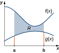
Figure 7. A region between two functions.
Again, we partition the interval [latex]\left[a,b\right][/latex] and construct rectangles. A representative rectangle is shown in the following figure.
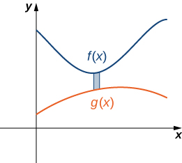
Figure 8. A representative rectangle of the region between two functions.
Note that the centroid of this rectangle is [latex]({x}_{i}^{*},(f({x}_{i}^{*})+g({x}_{i}^{*}))\text{/}2).[/latex] We won’t go through all the details of the Riemann sum development, but let’s look at some of the key steps. In the development of the formulas for the mass of the lamina and the moment with respect to the [latex]y[/latex]-axis, the height of each rectangle is given by [latex]f({x}_{i}^{*})-g({x}_{i}^{*}),[/latex] which leads to the expression [latex]f(x)-g(x)[/latex] in the integrands.
In the development of the formula for the moment with respect to the [latex]x[/latex]-axis, the moment of each rectangle is found by multiplying the area of the rectangle, [latex]\rho \left[f({x}_{i}^{*})-g({x}_{i}^{*})\right]\text{Δ}x,[/latex] by the distance of the centroid from the [latex]x[/latex]-axis, [latex](f({x}_{i}^{*})+g({x}_{i}^{*}))\text{/}2,[/latex] which gives [latex]\rho (1\text{/}2)\left\{{\left[f({x}_{i}^{*})\right]}^{2}-{\left[g({x}_{i}^{*})\right]}^{2}\right\}\text{Δ}x.[/latex] Summarizing these findings, we arrive at the following theorem.
Center of Mass of a Lamina Bounded by Two Functions
Let R denote a region bounded above by the graph of a continuous function [latex]f(x),[/latex] below by the graph of the continuous function [latex]g(x),[/latex] and on the left and right by the lines [latex]x=a[/latex] and [latex]x=b,[/latex] respectively. Let [latex]\rho[/latex] denote the density of the associated lamina. Then we can make the following statements:
- The mass of the lamina is
[latex]m=\rho {\displaystyle\int }_{a}^{b}\left[f(x)-g(x)\right]dx.[/latex]
- The moments [latex]{M}_{x}[/latex] and [latex]{M}_{y}[/latex] of the lamina with respect to the [latex]x[/latex]– and [latex]y[/latex]-axes, respectively, are
[latex]{M}_{x}=\rho {\displaystyle\int }_{a}^{b}\frac{1}{2}({\left[f(x)\right]}^{2}-{\left[g(x)\right]}^{2})dx\text{ and }{M}_{y}=\rho {\displaystyle\int }_{a}^{b}x\left[f(x)-g(x)\right]dx.[/latex]
- The coordinates of the center of mass [latex](\overline{x},\overline{y})[/latex] are
[latex]\overline{x}=\frac{{M}_{y}}{m}\text{ and }\overline{y}=\frac{{M}_{x}}{m}.[/latex]
We illustrate this theorem in the following example.
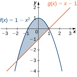
Example: Finding the Centroid of a Region Bounded by Two Functions
Let R be the region bounded above by the graph of the function [latex]f(x)=1-{x}^{2}[/latex] and below by the graph of the function [latex]g(x)=x-1.[/latex] Find the centroid of the region.
Try It
Let R be the region bounded above by the graph of the function [latex]f(x)=6-{x}^{2}[/latex] and below by the graph of the function [latex]g(x)=3-2x.[/latex] Find the centroid of the region.
Watch the following video to see the worked solution to the above Try It.
Try It
Candela Citations
- 2.6 Moments and Center of Mass. Authored by: Ryan Melton. License: CC BY: Attribution
- Calculus Volume 1. Authored by: Gilbert Strang, Edwin (Jed) Herman. Provided by: OpenStax. Located at: https://openstax.org/details/books/calculus-volume-1. License: CC BY-NC-SA: Attribution-NonCommercial-ShareAlike. License Terms: Access for free at https://openstax.org/books/calculus-volume-1/pages/1-introduction

Hint
Use the process from the previous example.