Learning Outcomes
- Recognize the meaning of the tangent to a curve at a point
- Calculate the slope of a tangent line
- Identify the derivative as the limit of a difference quotient
- Calculate the derivative of a given function at a point
Tangent Lines
We begin our study of calculus by revisiting the notion of secant lines and tangent lines. Recall that we used the slope of a secant line to a function at a point [latex](a,f(a))[/latex] to estimate the rate of change, or the rate at which one variable changes in relation to another variable. We can obtain the slope of the secant by choosing a value of [latex]x[/latex] near [latex]a[/latex] and drawing a line through the points [latex](a,f(a))[/latex] and [latex](x,f(x))[/latex], as shown in Figure 2. The slope of this line is given by an equation in the form of a difference quotient:
We can also calculate the slope of a secant line to a function at a value [latex]a[/latex] by using this equation and replacing [latex]x[/latex] with [latex]a+h[/latex], where [latex]h[/latex] is a value close to [latex]0[/latex]. We can then calculate the slope of the line through the points [latex](a,f(a))[/latex] and [latex](a+h,f(a+h))[/latex]. In this case, we find the secant line has a slope given by the following difference quotient with increment [latex]h[/latex]:
Definition
Let [latex]f[/latex] be a function defined on an interval [latex]I[/latex] containing [latex]a[/latex]. If [latex]x\ne a[/latex] is in [latex]I[/latex], then
is a difference quotient.
Also, if [latex]h\ne 0[/latex] is chosen so that [latex]a+h[/latex] is in [latex]I[/latex], then
is a difference quotient with increment [latex]h[/latex].
These two expressions for calculating the slope of a secant line are illustrated in Figure 2. We will see that each of these two methods for finding the slope of a secant line is of value. Depending on the setting, we can choose one or the other. The primary consideration in our choice usually depends on ease of calculation.
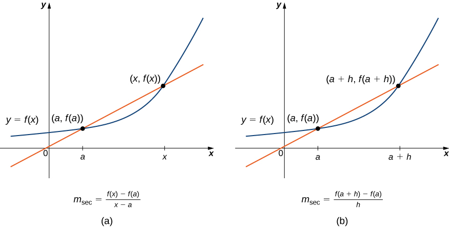
Figure 2. We can calculate the slope of a secant line in either of two ways.
In Figure 3(a) we see that, as the values of [latex]x[/latex] approach [latex]a[/latex], the slopes of the secant lines provide better estimates of the rate of change of the function at [latex]a[/latex]. Furthermore, the secant lines themselves approach the tangent line to the function at [latex]a[/latex], which represents the limit of the secant lines. Similarly, Figure 3(b) shows that as the values of [latex]h[/latex] get closer to 0, the secant lines also approach the tangent line. The slope of the tangent line at [latex]a[/latex] is the rate of change of the function at [latex]a[/latex], as shown in Figure 3(c).
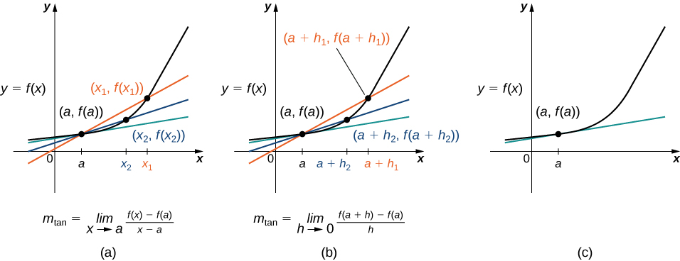
Figure 3. The secant lines approach the tangent line (shown in green) as the second point approaches the first.
In Figure 4, we show the graph of [latex]f(x)=\sqrt{x}[/latex] and its tangent line at [latex](1,1)[/latex] in a series of tighter intervals about [latex]x=1[/latex]. As the intervals become narrower, the graph of the function and its tangent line appear to coincide, making the values on the tangent line a good approximation to the values of the function for choices of [latex]x[/latex] close to 1. In fact, the graph of [latex]f(x)[/latex] itself appears to be locally linear in the immediate vicinity of [latex]x=1[/latex].
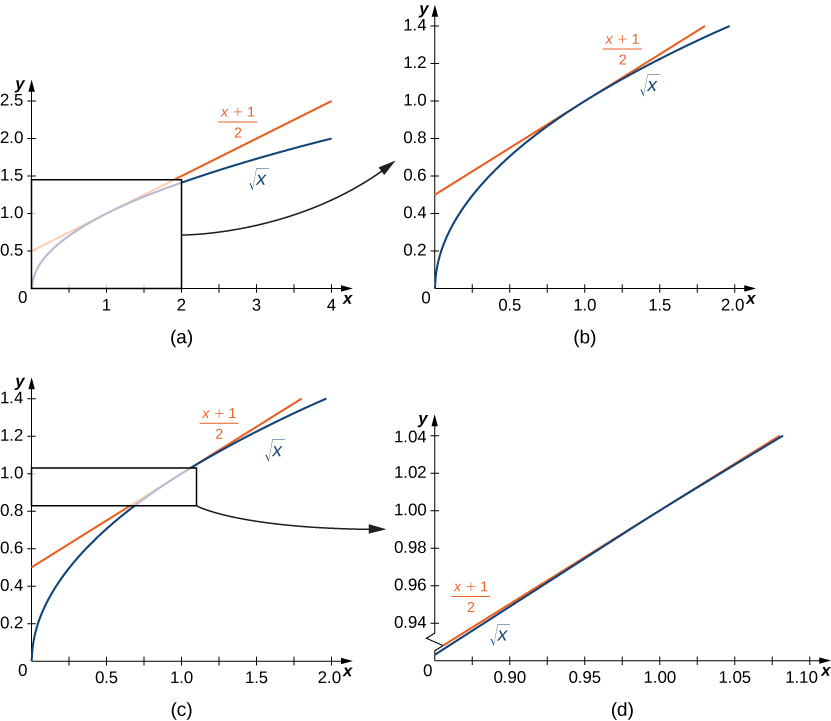
Figure 4. For values of [latex]x[/latex] close to 1, the graph of [latex]f(x)=\sqrt{x}[/latex] and its tangent line appear to coincide.
Formally we may define the tangent line to the graph of a function as follows.
Definition
Let [latex]f(x)[/latex] be a function defined in an open interval containing [latex]a[/latex]. The tangent line to [latex]f(x)[/latex] at [latex]a[/latex] is the line passing through the point [latex](a,f(a))[/latex] having slope
provided this limit exists.
Equivalently, we may define the tangent line to [latex]f(x)[/latex] at [latex]a[/latex] to be the line passing through the point [latex](a,f(a))[/latex] having slope
provided this limit exists.
Just as we have used two different expressions to define the slope of a secant line, we use two different forms to define the slope of the tangent line. In this text we use both forms of the definition. As before, the choice of definition will depend on the setting. Now that we have formally defined a tangent line to a function at a point, we can use this definition to find equations of tangent lines. The definition requires you to recall two algebraic techniques and formulas: evaluating a function with variable inputs and using point-slope form to write an equation of a line.
Recall: Evaluating a function with variable inputs
Functions can be evaluated for inputs that are variables or expressions. The process is the same as evaluating with a constant, but the simplified answer will contain a variable. The following examples show how to evaluate a function for a variable input.
Given [latex]f(x)=4x+1[/latex], find [latex]f(h+1)[/latex].
This time, you substitute [latex](h+1)[/latex] into the equation for x.
[latex]f(h+1)=4(h+1)+1[/latex]
Use the distributive property on the right side, and then combine like terms to simplify.
[latex]f(h+1)=4h+4+1=4h+5[/latex]
Given [latex]f(x)=4x+1[/latex], [latex]f(h+1)=4h+5[/latex].
Watch this video for more:
Recall: writing an equation of a line using point-slope form
Point-slope form of a linear equation takes the form
[latex]y-{y}_{1}=m\left(x-{x}_{1}\right)[/latex]
where [latex]m[/latex] is the slope and [latex]{x}_{1 }\text{ and } {y}_{1}[/latex] are the [latex]x\text{ and }y[/latex] coordinates of a specific point through which the line passes.
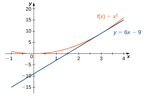
Example: Finding a Tangent Line
Find the equation of the line tangent to the graph of [latex]f(x)=x^2[/latex] at [latex]x=3[/latex].
Watch the following video to see the worked solution to Example: Finding a Tangent Line.
Example: The Slope of a Tangent Line Revisited
Use the second definition to find the slope of the line tangent to the graph of [latex]f(x)=x^2[/latex] at [latex]x=3[/latex].
Example: Finding the Equation of a Tangent Line
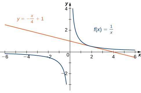
Find the equation of the line tangent to the graph of [latex]f(x)=\dfrac{1}{x}[/latex] at [latex]x=2[/latex].
Try It
Find the slope of the line tangent to the graph of [latex]f(x)=\sqrt{x}[/latex] at [latex]x=4[/latex].
Watch the following video to see the worked solution to the above Try It.
Try It
The Derivative of a Function at a Point
The type of limit we compute in order to find the slope of the line tangent to a function at a point occurs in many applications across many disciplines. These applications include velocity and acceleration in physics, marginal profit functions in business, and growth rates in biology. This limit occurs so frequently that we give this value a special name: the derivative. The process of finding a derivative is called differentiation.
Definition
Let [latex]f(x)[/latex] be a function defined in an open interval containing [latex]a[/latex]. The derivative of the function [latex]f(x)[/latex] at [latex]a[/latex], denoted by [latex]f^{\prime}(a)[/latex], is defined by
provided this limit exists.
Alternatively, we may also define the derivative of [latex]f(x)[/latex] at [latex]a[/latex] as
provided this limit exists.
Example: Estimating a Derivative
For [latex]f(x)=x^2[/latex], use a table to estimate [latex]f^{\prime}(3)[/latex] using the first definition above.
Try It
For [latex]f(x)=x^2[/latex], use a table to estimate [latex]f^{\prime}(3)[/latex] using the second definition.
Example: Finding a Derivative
For [latex]f(x)=3x^2-4x+1[/latex], find [latex]f^{\prime}(2)[/latex] by using the first definition.
Example: Revisiting the Derivative
For [latex]f(x)=3x^2-4x+1[/latex], find [latex]f^{\prime}(2)[/latex] by using the second definition.
Try It
For [latex]f(x)=x^2+3x+2[/latex], find [latex]f^{\prime}(1)[/latex].
Watch the following video to see the worked solution to the above Try It.
Try It
Candela Citations
- 3.1 Defining the Derivative. Authored by: Ryan Melton. License: CC BY: Attribution
- Calculus Volume 1. Authored by: Gilbert Strang, Edwin (Jed) Herman. Provided by: OpenStax. Located at: https://openstax.org/details/books/calculus-volume-1. License: CC BY-NC-SA: Attribution-NonCommercial-ShareAlike. License Terms: Access for free at https://openstax.org/books/calculus-volume-1/pages/1-introduction
