Derivative of the Exponential Function

Just as when we found the derivatives of other functions, we can find the derivatives of exponential and logarithmic functions using formulas. As we develop these formulas, we need to make certain basic assumptions. The proofs that these assumptions hold are beyond the scope of this course.

First of all, we begin with the assumption that the function [latex]B(x)=b^x, \, b>0[/latex], is defined for every real number and is continuous. In previous courses, the values of exponential functions for all rational numbers were defined—beginning with the definition of [latex]b^n[/latex], where [latex]n[/latex] is a positive integer—as the product of [latex]b[/latex] multiplied by itself [latex]n[/latex] times. Later, we defined [latex]b^0=1, \, b^{−n}=\frac{1}{b^n}[/latex] for a positive integer [latex]n[/latex], and [latex]b^{s/t}=(\sqrt[t]{b})^s[/latex] for positive integers [latex]s[/latex] and [latex]t[/latex]. These definitions leave open the question of the value of [latex]b^r[/latex] where [latex]r[/latex] is an arbitrary real number. By assuming the continuity of [latex]B(x)=b^x, \, b>0[/latex], we may interpret [latex]b^r[/latex] as [latex]\underset{x\to r}{\lim}b^x[/latex] where the values of [latex]x[/latex] as we take the limit are rational. For example, we may view [latex]{4}^{\pi}[/latex] as the number satisfying

As we see in the following table, [latex]4^{\pi}\approx 77.88[/latex].

We also assume that for [latex]B(x)=b^x, \, b>0[/latex], the value [latex]B^{\prime}(0)[/latex] of the derivative exists. In this section, we show that by making this one additional assumption, it is possible to prove that the function [latex]B(x)[/latex] is differentiable everywhere.

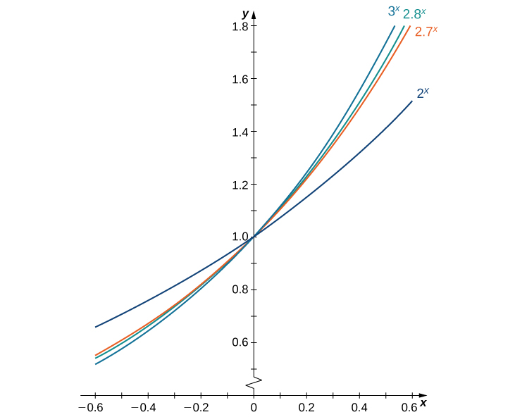
We make one final assumption: that there is a unique value of [latex]b>0[/latex] for which [latex]B^{\prime}(0)=1[/latex]. We define [latex]e[/latex] to be this unique value, as we did in Introduction to Functions and Graphs. Figure 1 provides graphs of the functions [latex]y=2^x, \, y=3^x, \, y=2.7^x[/latex], and [latex]y=2.8^x[/latex]. A visual estimate of the slopes of the tangent lines to these functions at 0 provides evidence that the value of [latex]e[/latex] lies somewhere between 2.7 and 2.8. The function [latex]E(x)=e^x[/latex] is called the natural exponential function. Its inverse, [latex]L(x)=\log_e x=\ln x[/latex] is called the natural logarithmic function.

Figure 1. The graph of [latex]E(x)=e^x[/latex] is between [latex]y=2^x[/latex] and [latex]y=3^x[/latex].

For a better estimate of [latex]e[/latex], we may construct a table of estimates of [latex]B^{\prime}(0)[/latex] for functions of the form [latex]B(x)=b^x[/latex]. Before doing this, recall that

for values of [latex]x[/latex] very close to zero. For our estimates, we choose [latex]x=0.00001[/latex] and [latex]x=-0.00001[/latex] to obtain the estimate

[latex]\dfrac{b^{-0.00001}-1}{-0.00001}

 

See the following table.

Estimating a Value of [latex]e[/latex]

[latex]b[/latex]	[latex]\frac{b^{-0.00001}-1}{-0.00001}	[latex]b[/latex]	[latex]\frac{b^{-0.00001}-1}{-0.00001}
2	[latex]0.693145	2.7183	[latex]1.000002
2.7	[latex]0.993247	2.719	[latex]1.000259
2.71	[latex]0.996944	2.72	[latex]1.000627
2.718	[latex]0.999891	2.8	[latex]1.029614
2.7182	[latex]0.999965	3	[latex]1.098606

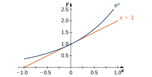
The evidence from the table suggests that [latex]2.7182

The graph of [latex]E(x)=e^x[/latex] together with the line [latex]y=x+1[/latex] are shown in Figure 2. This line is tangent to the graph of [latex]E(x)=e^x[/latex] at [latex]x=0[/latex].

 

Figure 2. The tangent line to [latex]E(x)=e^x[/latex] at [latex]x=0[/latex] has slope 1.

Now that we have laid out our basic assumptions, we begin our investigation by exploring the derivative of [latex]B(x)=b^x, \, b>0[/latex]. Recall that we have assumed that [latex]B^{\prime}(0)[/latex] exists. By applying the limit definition to the derivative we conclude that

[latex]B^{\prime}(0)=\underset{h\to 0}{\lim}\dfrac{b^{0+h}-b^0}{h}=\underset{h\to 0}{\lim}\dfrac{b^h-1}{h}[/latex]

 

Turning to [latex]B^{\prime}(x)[/latex], we obtain the following.

[latex]\begin{array}{lllll} B^{\prime}(x) & =\underset{h\to 0}{\lim}\frac{b^{x+h}-b^x}{h} & & & \text{Apply the limit definition of the derivative.} \\ & =\underset{h\to 0}{\lim}\frac{b^xb^h-b^x}{h} & & & \text{Note that} \, b^{x+h}=b^x b^h. \\ & =\underset{h\to 0}{\lim}\frac{b^x(b^h-1)}{h} & & & \text{Factor out} \, b^x. \\ & =b^x\underset{h\to 0}{\lim}\frac{b^h-1}{h} & & & \text{Apply a property of limits.} \\ & =b^x B^{\prime}(0) & & & \text{Use} \, B^{\prime}(0)=\underset{h\to 0}{\lim}\frac{b^{0+h}-b^0}{h}=\underset{h\to 0}{\lim}\frac{b^h-1}{h}. \end{array}[/latex]

 

We see that on the basis of the assumption that [latex]B(x)=b^x[/latex] is differentiable at [latex]0, \, B(x)[/latex] is not only differentiable everywhere, but its derivative is

[latex]B^{\prime}(x)=b^x B^{\prime}(0)[/latex]

 

For [latex]E(x)=e^x, \, E^{\prime}(0)=1[/latex]. Thus, we have [latex]E^{\prime}(x)=e^x[/latex]. (The value of [latex]B^{\prime}(0)[/latex] for an arbitrary function of the form [latex]B(x)=b^x, \, b>0[/latex], will be derived later.)

Derivative of the Natural Exponential Function

---

Let [latex]E(x)=e^x[/latex] be the natural exponential function. Then

[latex]E^{\prime}(x)=e^x[/latex]

 

In general,

[latex]\frac{d}{dx}(e^{g(x)})=e^{g(x)} g^{\prime}(x)[/latex]

If it helps, think of the formula as the chain rule being applied to natural exponential functions. The derivative of [latex]{e}[/latex] raised to the power of a function will simply be [latex]{e}[/latex] raised to the power of the function multiplied by the derivative of that function.

Example: Derivative of an Exponential Function

Find the derivative of [latex]f(x)=e^{\tan (2x)}[/latex].

Show Solution

Using the derivative formula and the chain rule,

[latex]\begin{array}{ll} f^{\prime}(x) & =e^{\tan (2x)}\frac{d}{dx}(\tan (2x)) \\ & = e^{\tan (2x)} \sec^2 (2x) \cdot 2. \end{array}[/latex]

 

Example: Combining Differentiation Rules

Find the derivative of [latex]y=\dfrac{e^{x^2}}{x}[/latex].

Show Solution

Use the derivative of the natural exponential function, the quotient rule, and the chain rule.

[latex]\begin{array}{lllll} y^{\prime} & =\large \frac{(e^{x^2} \cdot 2x) \cdot x - 1 \cdot e^{x^2}}{x^2} & & & \text{Apply the quotient rule.} \\ & = \large \frac{e^{x^2}(2x^2-1)}{x^2} & & & \text{Simplify.} \end{array}[/latex]

 

Try It

Find the derivative of [latex]h(x)=xe^{2x}[/latex].

Hint

Don’t forget to use the product rule.

Show Solution

[latex]h^{\prime}(x)=e^{2x}+2xe^{2x}[/latex]

Watch the following video to see the worked solution to the above Try It.

Closed Captioning and Transcript Information for Video

For closed captioning, open the video on its original page by clicking the Youtube logo in the lower right-hand corner of the video display. In YouTube, the video will begin at the same starting point as this clip, but will continue playing until the very end.

You can view the transcript for this segmented clip of “3.9 Derivatives of Exponential and Logarithmic Functions” here (opens in new window).

Try It

Example: Applying the Natural Exponential Function

A colony of mosquitoes has an initial population of 1000. After [latex]t[/latex] days, the population is given by [latex]A(t)=1000e^{0.3t}[/latex]. Show that the ratio of the rate of change of the population, [latex]A^{\prime}(t)[/latex], to the population size, [latex]A(t)[/latex] is constant.

Show Solution

First find [latex]A^{\prime}(t)[/latex]. By using the chain rule, we have [latex]A^{\prime}(t)=300e^{0.3t}[/latex]. Thus, the ratio of the rate of change of the population to the population size is given by

[latex]\large \frac{A^{\prime}(t)}{A(t)} \normalsize = \large \frac{300e^{0.3t}}{1000e^{0.3t}}=0.3[/latex]

 

The ratio of the rate of change of the population to the population size is the constant 0.3.

Watch the following video to see the worked solution to Example: Applying the Natural Exponential Function.

Closed Captioning and Transcript Information for Video

For closed captioning, open the video on its original page by clicking the Youtube logo in the lower right-hand corner of the video display. In YouTube, the video will begin at the same starting point as this clip, but will continue playing until the very end.

You can view the transcript for this segmented clip of “3.9 Derivatives of Exponential and Logarithmic Functions” here (opens in new window).

Try It

If [latex]A(t)=1000e^{0.3t}[/latex] describes the mosquito population after [latex]t[/latex] days, as in the preceding example, what is the rate of change of [latex]A(t)[/latex] after 4 days?

Hint

Find [latex]A^{\prime}(4)[/latex].

Show Solution

996