Learning Outcomes
- Analyze a function and its derivatives to draw its graph
Guidelines for Graphing a Function
We now have enough analytical tools to draw graphs of a wide variety of algebraic and transcendental functions. Before showing how to graph specific functions, let’s look at a general strategy to use when graphing any function.
Problem-Solving Strategy: Drawing the Graph of a Function
Given a function [latex]f[/latex] use the following steps to sketch a graph of [latex]f[/latex]:
- Determine the domain of the function.
- Locate the [latex]x[/latex]– and [latex]y[/latex]-intercepts.
- Evaluate [latex]\underset{x\to \infty }{\lim}f(x)[/latex] and [latex]\underset{x\to −\infty }{\lim}f(x)[/latex] to determine the end behavior. If either of these limits is a finite number [latex]L[/latex], then [latex]y=L[/latex] is a horizontal asymptote. If either of these limits is [latex]\infty[/latex] or [latex]−\infty[/latex], determine whether [latex]f[/latex] has an oblique asymptote. If [latex]f[/latex] is a rational function such that [latex]f(x)=\frac{p(x)}{q(x)}[/latex], where the degree of the numerator is greater than the degree of the denominator, then [latex]f[/latex] can be written as
[latex]f(x)=\dfrac{p(x)}{q(x)}=g(x)+\dfrac{r(x)}{q(x)}[/latex],
where the degree of [latex]r(x)[/latex] is less than the degree of [latex]q(x)[/latex]. The values of [latex]f(x)[/latex] approach the values of [latex]g(x)[/latex] as [latex]x\to \pm \infty[/latex]. If [latex]g(x)[/latex] is a linear function, it is known as an oblique asymptote.
- Determine whether [latex]f[/latex] has any vertical asymptotes.
- Calculate [latex]f^{\prime}[/latex]. Find all critical points and determine the intervals where [latex]f[/latex] is increasing and where [latex]f[/latex] is decreasing. Determine whether [latex]f[/latex] has any local extrema.
- Calculate [latex]f^{\prime \prime}[/latex]. Determine the intervals where [latex]f[/latex] is concave up and where [latex]f[/latex] is concave down. Use this information to determine whether [latex]f[/latex] has any inflection points. The second derivative can also be used as an alternate means to determine or verify that [latex]f[/latex] has a local extremum at a critical point.
Now let’s use this strategy to graph several different functions. We start by graphing a polynomial function.
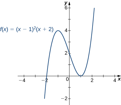
Example: Sketching a Graph of a Polynomial
Sketch a graph of [latex]f(x)=(x-1)^2 (x+2)[/latex]
Watch the following video to see the worked solution to Example: Sketching a Graph of a Polynomial.
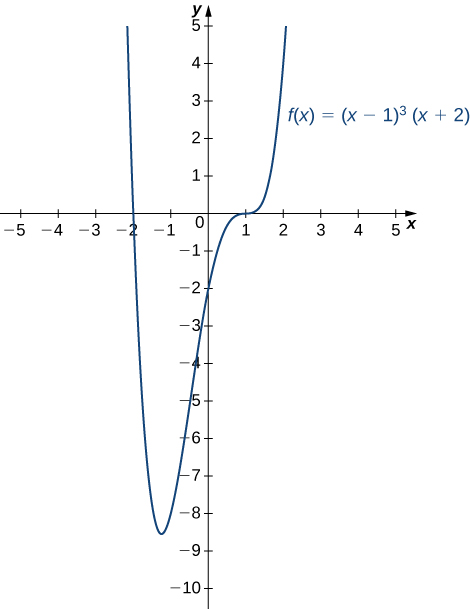
Try It
Sketch a graph of [latex]f(x)=(x-1)^3 (x+2)[/latex]
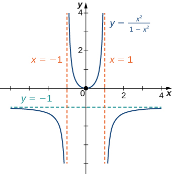
Example: Sketching a Rational Function
Sketch the graph of [latex]f(x)=\dfrac{x^2}{1-x^2}[/latex]
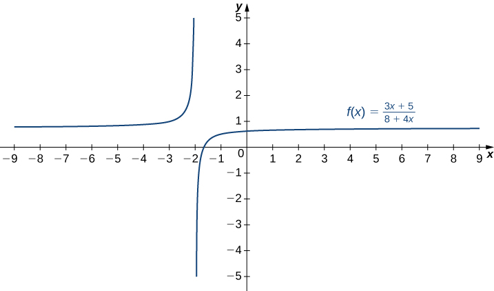
Try It
Sketch a graph of [latex]f(x)=\dfrac{3x+5}{8+4x}[/latex]
Example: Sketching a Rational Function with an Oblique Asymptote
Sketch the graph of [latex]f(x)=\dfrac{x^2}{x-1}[/latex]
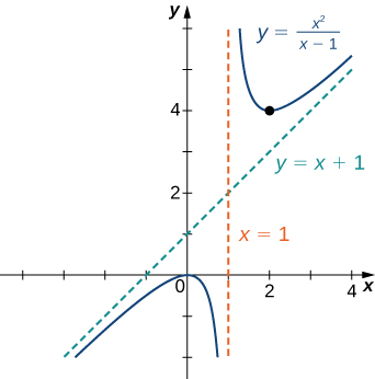
Watch the following video to see the worked solution to Example: Sketching a Rational Function with an Oblique Asymptote.
Try It
Find the oblique asymptote for [latex]f(x)=\dfrac{3x^3-2x+1}{2x^2-4}[/latex]
Use long division of polynomials.
Example: Sketching the Graph of a Function with a Cusp
Sketch a graph of [latex]f(x)=(x-1)^{\frac{2}{3}}[/latex]
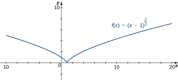
Watch the following video to see the worked solution to Example: Sketching the Graph of a Function with a Cusp.
Try It
Consider the function [latex]f(x)=5-x^{\frac{2}{3}}[/latex]. Determine the point on the graph where a cusp is located. Determine the end behavior of [latex]f[/latex].
Candela Citations
- 4.6 Limits at Infinity and Asymptotes (part 2 - curve sketching). Authored by: Ryan Melton. License: CC BY: Attribution
- Calculus Volume 1. Authored by: Gilbert Strang, Edwin (Jed) Herman. Provided by: OpenStax. Located at: https://openstax.org/details/books/calculus-volume-1. License: CC BY-NC-SA: Attribution-NonCommercial-ShareAlike. License Terms: Access for free at https://openstax.org/books/calculus-volume-1/pages/1-introduction
