Learning Outcomes
- Identify the graphs and periods of the trigonometric functions
- Describe the shift of a sine or cosine graph from the equation of the function
We have seen that as we travel around the unit circle, the values of the trigonometric functions repeat. We can see this pattern in the graphs of the functions. Let [latex]P=(x,y)[/latex] be a point on the unit circle and let [latex]\theta[/latex] be the corresponding angle. Since the angle [latex]\theta[/latex] and [latex]\theta +2\pi[/latex] correspond to the same point [latex]P[/latex], the values of the trigonometric functions at [latex]\theta[/latex] and at [latex]\theta +2\pi[/latex] are the same. Consequently, the trigonometric functions are periodic functions. The period of a function [latex]f[/latex] is defined to be the smallest positive value [latex]p[/latex] such that [latex]f(x+p)=f(x)[/latex] for all values [latex]x[/latex] in the domain of [latex]f[/latex]. The sine, cosine, secant, and cosecant functions have a period of [latex]2\pi[/latex]. Since the tangent and cotangent functions repeat on an interval of length [latex]\pi[/latex], their period is [latex]\pi[/latex] (Figure 9).
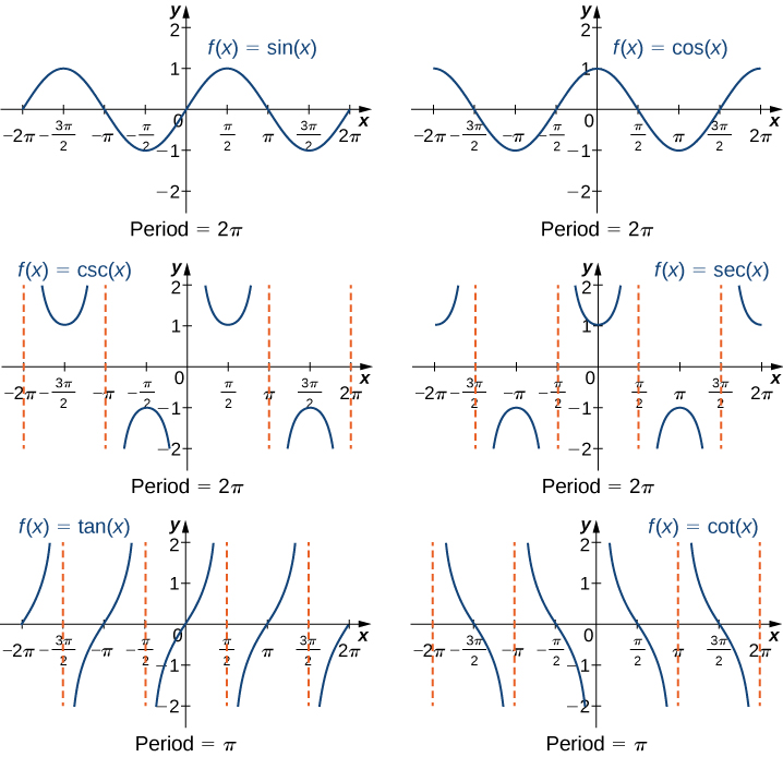
Figure 9. The six trigonometric functions are periodic.
Try It
Transformations to Trigonometric Graphs
Just as with algebraic functions, we can apply transformations to trigonometric functions. In particular, consider the following function:
In Figure 10, the constant [latex]\alpha[/latex] causes a horizontal or phase shift. The factor [latex]B[/latex] changes the period. This transformed sine function will have a period [latex]2\pi / |B|[/latex]. The factor [latex]A[/latex] results in a vertical stretch by a factor of [latex]|A|[/latex]. We say [latex]|A|[/latex] is the “amplitude of [latex]f[/latex].” The constant [latex]C[/latex] causes a vertical shift.
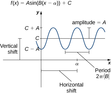
Figure 10. A graph of a general sine function.
Notice in Figure 9 that the graph of [latex]y=\cos x[/latex] is the graph of [latex]y=\sin x[/latex] shifted to the left [latex]\pi /2[/latex] units. Therefore, we can write [latex]\cos x=\sin(x+\pi /2)[/latex]. Similarly, we can view the graph of [latex]y=\sin x[/latex] as the graph of [latex]y=\cos x[/latex] shifted right [latex]\pi /2[/latex] units, and state that [latex]\sin x=\cos(x-\pi /2)[/latex].
A shifted sine curve arises naturally when graphing the number of hours of daylight in a given location as a function of the day of the year. For example, suppose a city reports that June 21 is the longest day of the year with 15.7 hours and December 21 is the shortest day of the year with 8.3 hours. It can be shown that the function
is a model for the number of hours of daylight [latex]h[/latex] as a function of day of the year [latex]t[/latex] (Figure 11).
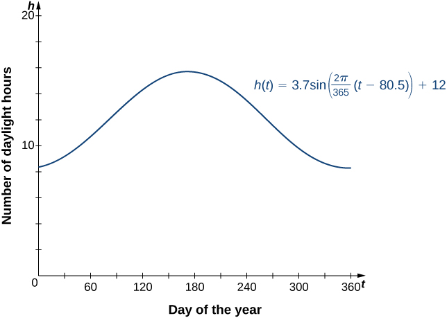
Figure 11. The hours of daylight as a function of day of the year can be modeled by a shifted sine curve.
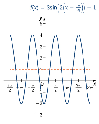
Example: Sketching the Graph of a Transformed Sine Curve
Sketch a graph of [latex]f(x)=3\sin(2(x-\frac{\pi}{4}))+1[/latex].
Watch the following video to see the worked solution to Example: Sketching the Graph of a Transformed Sine Curve
Try It
Describe the relationship between the graph of [latex]f(x)=3\sin(4x)-5[/latex] and the graph of [latex]y=\sin x[/latex].
Try It
Candela Citations
- 1.3.4. Authored by: Ryan Melton. License: CC BY: Attribution
- Calculus Volume 1. Authored by: Gilbert Strang, Edwin (Jed) Herman. Provided by: OpenStax. Located at: https://openstax.org/details/books/calculus-volume-1. License: CC BY-NC-SA: Attribution-NonCommercial-ShareAlike. License Terms: Access for free at https://openstax.org/books/calculus-volume-1/pages/1-introduction
