Learning Outcomes
- Determine the conditions for when a function has an inverse
- Use the horizontal line test to recognize when a function is one-to-one
- Find the inverse of a given function
- Draw the graph of an inverse function
Existence of an Inverse Function
We begin with an example. Given a function [latex]f[/latex] and an output [latex]y=f(x)[/latex], we are often interested in finding what value or values [latex]x[/latex] were mapped to [latex]y[/latex] by [latex]f[/latex]. For example, consider the function [latex]f(x)=x^3+4[/latex]. Since any output [latex]y=x^3+4[/latex], we can solve this equation for [latex]x[/latex] to find that the input is [latex]x=\sqrt[3]{y-4}[/latex]. This equation defines [latex]x[/latex] as a function of [latex]y[/latex]. Denoting this function as [latex]f^{-1}[/latex], and writing [latex]x=f^{-1}(y)=\sqrt[3]{y-4}[/latex], we see that for any [latex]x[/latex] in the domain of [latex]f, \, f^{-1}(f(x))=f^{-1}(x^3+4)=x[/latex]. Thus, this new function, [latex]f^{-1}[/latex], “undid” what the original function [latex]f[/latex] did. A function with this property is called the inverse function of the original function.
Definition
Given a function [latex]f[/latex] with domain [latex]D[/latex] and range [latex]R[/latex], its inverse function (if it exists) is the function [latex]f^{-1}[/latex] with domain [latex]R[/latex] and range [latex]D[/latex] such that [latex]f^{-1}(y)=x[/latex] if [latex]f(x)=y[/latex]. In other words, for a function [latex]f[/latex] and its inverse [latex]f^{-1}[/latex],
Note that [latex]f^{-1}[/latex] is read as “f inverse.” Here, the -1 is not used as an exponent and [latex]f^{-1}(x) \ne 1/f(x)[/latex]. Figure 1 shows the relationship between the domain and range of [latex]f[/latex] and the domain and range of [latex]f^{-1}[/latex].
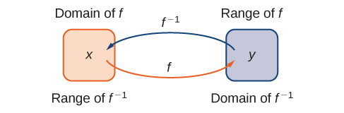
Figure 1. Given a function [latex]f[/latex] and its inverse [latex]f^{-1}, \, f^{-1}(y)=x[/latex] if and only if [latex]f(x)=y[/latex]. The range of [latex]f[/latex] becomes the domain of [latex]f^{-1}[/latex] and the domain of [latex]f[/latex] becomes the range of [latex]f^{-1}[/latex].
Recall that a function has exactly one output for each input. Remember the vertical line test?
Recall: THe vertical line test
We can identify whether the graph of a relation represents a function because for each [latex]x[/latex]-coordinate there will be exactly one [latex]y[/latex]-coordinate.
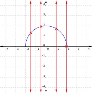
Figure 2. Semicircle graph undergoing the vertical line test.
When a vertical line is placed across the plot of this relation, it does not intersect the graph more than once for any values of [latex]x[/latex]. This is a graph of a function.
If, on the other hand, a graph shows two or more intersections with a vertical line, then an input ([latex]x[/latex]-coordinate) can have more than one output ([latex]y[/latex]-coordinate), and [latex]y[/latex] is not a function of [latex]x[/latex]. Examining the graph of a relation to determine if a vertical line would intersect with more than one point is a quick way to determine if the relation shown by the graph is a function.
Therefore, to define an inverse function, we need to map each input to exactly one output. For example, let’s try to find the inverse function for [latex]f(x)=x^2[/latex]. Solving the equation [latex]y=x^2[/latex] for [latex]x[/latex], we arrive at the equation [latex]x= \pm \sqrt{y}[/latex]. This equation does not describe [latex]x[/latex] as a function of [latex]y[/latex] because there are two solutions to this equation for every [latex]y>0[/latex]. The problem with trying to find an inverse function for [latex]f(x)=x^2[/latex] is that two inputs are sent to the same output for each output [latex]y>0[/latex]. The function [latex]f(x)=x^3+4[/latex] discussed earlier did not have this problem. For that function, each input was sent to a different output. A function that sends each input to a different output is called a one-to-one function.
Try It
Definition
We say a [latex]f[/latex] is a one-to-one function if [latex]f(x_1) \ne f(x_2)[/latex] when [latex]x_1 \ne x_2[/latex].
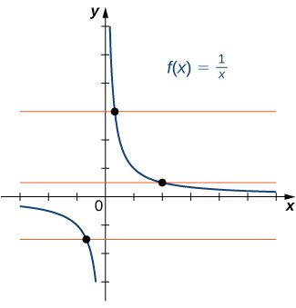
One way to determine whether a function is one-to-one is by looking at its graph. If a function is one-to-one, then no two inputs can be sent to the same output. Therefore, if we draw a horizontal line anywhere in the [latex]xy[/latex]-plane, according to the horizontal line test, it cannot intersect the graph more than once. We note that the horizontal line test is different from the vertical line test. The vertical line test determines whether a graph is the graph of a function. The horizontal line test determines whether a function is one-to-one (Figure 3).
Horizontal Line Test
A function [latex]f[/latex] is one-to-one if and only if every horizontal line intersects the graph of [latex]f[/latex] no more than once.
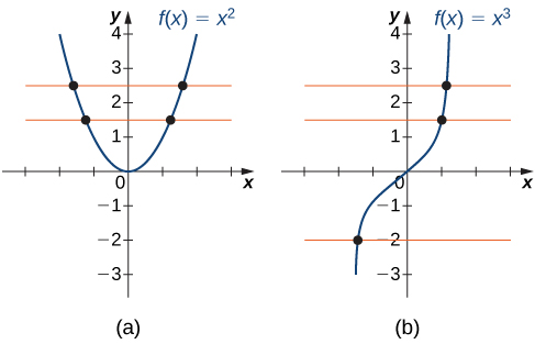
Figure 3. (a) The function [latex]f(x)=x^2[/latex] is not one-to-one because it fails the horizontal line test. (b) The function [latex]f(x)=x^3[/latex] is one-to-one because it passes the horizontal line test.
Example: Determining Whether a Function Is One-to-One
For each of the following functions, use the horizontal line test to determine whether it is one-to-one.
a.
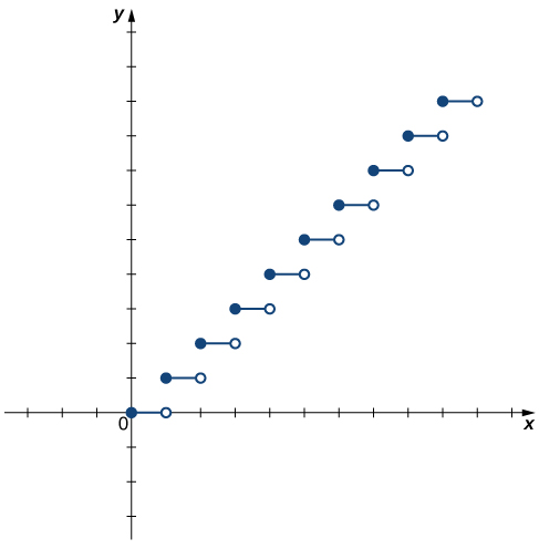
Figure 4. Is this function one-to-one?
b.
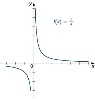
Figure 5. Is this function one-to-one?
Try It
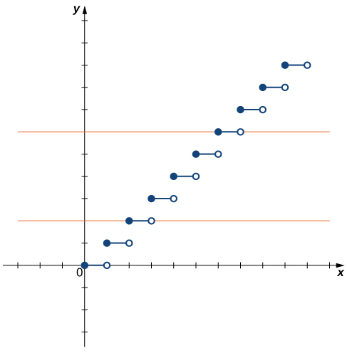
Is the function [latex]f[/latex] graphed in the following image one-to-one?
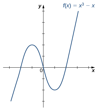
Figure 8. Is this function one-to-one?
Try It
Finding a Function’s Inverse
We can now consider one-to-one functions and show how to find their inverses. Recall that a function maps elements in the domain of [latex]f[/latex] to elements in the range of [latex]f[/latex]. The inverse function maps each element from the range of [latex]f[/latex] back to its corresponding element from the domain of [latex]f[/latex]. Therefore, to find the inverse function of a one-to-one function [latex]f[/latex], given any [latex]y[/latex] in the range of [latex]f[/latex], we need to determine which [latex]x[/latex] in the domain of [latex]f[/latex] satisfies [latex]f(x)=y[/latex]. Since [latex]f[/latex] is one-to-one, there is exactly one such value [latex]x[/latex]. We can find that value [latex]x[/latex] by solving the equation [latex]f(x)=y[/latex] for [latex]x[/latex]. Doing so, we are able to write [latex]x[/latex] as a function of [latex]y[/latex] where the domain of this function is the range of [latex]f[/latex] and the range of this new function is the domain of [latex]f[/latex]. Consequently, this function is the inverse of [latex]f[/latex], and we write [latex]x=f^{-1}(y)[/latex]. Since we typically use the variable [latex]x[/latex] to denote the independent variable and [latex]y[/latex] to denote the dependent variable, we often interchange the roles of [latex]x[/latex] and [latex]y[/latex], and write [latex]y=f^{-1}(x)[/latex]. Representing the inverse function in this way is also helpful later when we graph a function [latex]f[/latex] and its inverse [latex]f^{-1}[/latex] on the same axes.
Problem-Solving Strategy, Finding an Inverse Function
- Solve the equation [latex]y=f(x)[/latex] for [latex]x[/latex].
- Interchange the variables [latex]x[/latex] and [latex]y[/latex] and write [latex]y=f^{-1}(x)[/latex].
To complete the first step to finding an inverse function, we recall isolating a variable in a given equation.
Recall: isolate a variable in a formula
Isolate the variable for width [latex]w[/latex] from the formula for the perimeter of a rectangle:
[latex]{P}=2\left({l}\right)+2\left({w}\right)[/latex].
First, isolate the term with [latex]w[/latex] by subtracting [latex]2l[/latex] from both sides of the equation.
[latex]\displaystyle \begin{array}{l}\,\,\,\,\,\,\,\,\,\,P\,=\,\,\,\,2l+2w\\\underline{\,\,\,\,\,-2l\,\,\,\,\,-2l\,\,\,\,\,\,\,\,\,\,\,}\\P-2l=\,\,\,\,\,\,\,\,\,\,\,\,\,2w\end{array}[/latex]
Next, clear the coefficient of [latex]w[/latex] by dividing both sides of the equation by [latex]2[/latex].
[latex]\displaystyle \begin{array}{l}\underline{P-2l}=\underline{2w}\\\,\,\,\,\,\,2\,\,\,\,\,\,\,\,\,\,\,\,\,\,\,\,2\\ \,\,\,\dfrac{P-2l}{2}\,\,=\,\,w\\\,\,\,\,\,\,\,\,\,\,\,w=\dfrac{P-2l}{2}\end{array}[/latex]
You can rewrite the equation so the isolated variable is on the left side.
[latex]w=\Large\frac{P-2l}{2}[/latex]
Example: Finding an Inverse Function
Find the inverse for the function [latex]f(x)=3x-4[/latex]. State the domain and range of the inverse function. Verify that [latex]f^{-1}(f(x))=x[/latex].
Watch the following video to see the worked solution to Example: Finding an Inverse Function
Try It
Find the inverse of the function [latex]f(x)=\dfrac{3x}{(x-2)}[/latex]. State the domain and range of the inverse function.
Try It
Graphing Inverse Functions
Let’s consider the relationship between the graph of a function [latex]f[/latex] and the graph of its inverse. Consider the graph of [latex]f[/latex] shown in Figure 9(a) and a point [latex](a,b)[/latex] on the graph. Since [latex]b=f(a)[/latex], then [latex]f^{-1}(b)=a[/latex]. Therefore, when we graph [latex]f^{-1}[/latex], the point [latex](b,a)[/latex] is on the graph. As a result, the graph of [latex]f^{-1}[/latex] is a reflection of the graph of [latex]f[/latex] about the line [latex]y=x[/latex].
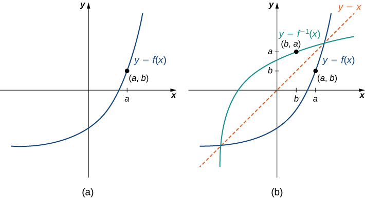
Figure 9. (a) The graph of this function [latex]f[/latex] shows point [latex](a,b)[/latex] on the graph of [latex]f[/latex]. (b) Since [latex](a,b)[/latex] is on the graph of [latex]f[/latex], the point [latex](b,a)[/latex] is on the graph of [latex]f^{-1}[/latex]. The graph of [latex]f^{-1}[/latex] is a reflection of the graph of [latex]f[/latex] about the line [latex]y=x[/latex].
Example: Sketching Graphs of Inverse Functions
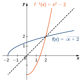
For the graph of [latex]f[/latex] in the following image, sketch a graph of [latex]f^{-1}[/latex] by sketching the line [latex]y=x[/latex] and using symmetry. Identify the domain and range of [latex]f^{-1}[/latex].
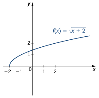
Figure 10. Graph of [latex]f(x)[/latex].
Try It
Sketch the graph of [latex]f(x)=2x+3[/latex] and the graph of its inverse using the symmetry property of inverse functions.
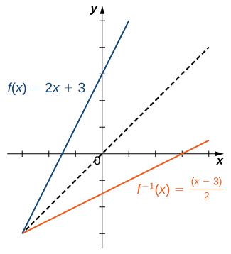
Try It
Restricting Domains
As we have seen, [latex]f(x)=x^2[/latex] does not have an inverse function because it is not one-to-one. However, we can choose a subset of the domain of [latex]f[/latex] such that the function is one-to-one. This subset is called a restricted domain. By restricting the domain of [latex]f[/latex], we can define a new function [latex]g[/latex] such that the domain of [latex]g[/latex] is the restricted domain of [latex]f[/latex] and [latex]g(x)=f(x)[/latex] for all [latex]x[/latex] in the domain of [latex]g[/latex]. Then we can define an inverse function for [latex]g[/latex] on that domain. For example, since [latex]f(x)=x^2[/latex] is one-to-one on the interval [latex][0,\infty)[/latex], we can define a new function [latex]g[/latex] such that the domain of [latex]g[/latex] is [latex][0,\infty)[/latex] and [latex]g(x)=x^2[/latex] for all [latex]x[/latex] in its domain. Since [latex]g[/latex] is a one-to-one function, it has an inverse function, given by the formula [latex]g^{-1}(x)=\sqrt{x}[/latex]. On the other hand, the function [latex]f(x)=x^2[/latex] is also one-to-one on the domain [latex](−\infty,0][/latex]. Therefore, we could also define a new function [latex]h[/latex] such that the domain of [latex]h[/latex] is [latex](−\infty,0][/latex] and [latex]h(x)=x^2[/latex] for all [latex]x[/latex] in the domain of [latex]h[/latex]. Then [latex]h[/latex] is a one-to-one function and must also have an inverse. Its inverse is given by the formula [latex]h^{-1}(x)=−\sqrt{x}[/latex] (Figure 13).
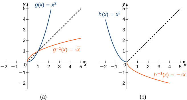
Figure 13. (a) For [latex]g(x)=x^2[/latex] restricted to [latex][0,\infty), \, g^{-1}(x)=\sqrt{x}[/latex]. (b) For [latex]h(x)=x^2[/latex] restricted to [latex](−\infty,0], \, h^{-1}(x)=−\sqrt{x}[/latex].
Example: Restricting the Domain
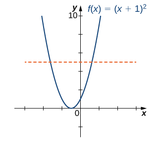
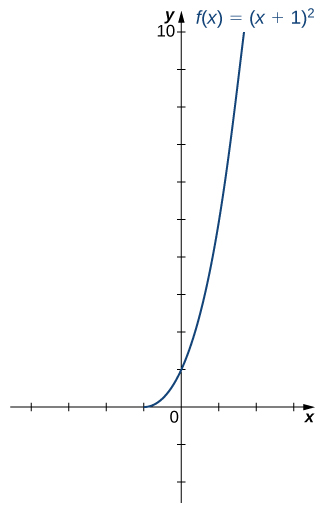
Consider the function [latex]f(x)=(x+1)^2[/latex].
- Sketch the graph of [latex]f[/latex] and use the horizontal line test to show that [latex]f[/latex] is not one-to-one.
- Show that [latex]f[/latex] is one-to-one on the restricted domain [latex][-1,\infty)[/latex]. Determine the domain and range for the inverse of [latex]f[/latex] on this restricted domain and find a formula for [latex]f^{-1}[/latex].
Watch the following video to see the worked solution to Example: Restricting the Domain
Try It
Consider [latex]f(x)=\dfrac{1}{x^2}[/latex] restricted to the domain [latex](−\infty ,0)[/latex]. Verify that [latex]f[/latex] is one-to-one on this domain. Determine the domain and range of the inverse of [latex]f[/latex] and find a formula for [latex]f^{-1}[/latex].
Candela Citations
- 1.4 Inverse Functions. Authored by: Ryan Melton. License: CC BY: Attribution
- Calculus Volume 1. Authored by: Gilbert Strang, Edwin (Jed) Herman. Provided by: OpenStax. Located at: https://openstax.org/details/books/calculus-volume-1. License: CC BY-NC-SA: Attribution-NonCommercial-ShareAlike. License Terms: Access for free at https://openstax.org/books/calculus-volume-1/pages/1-introduction
