We begin by examining what it means for a function to have a finite limit at infinity. Then we study the idea of a function with an infinite limit at infinity. We have looked at vertical asymptotes in other modules; in this section, we deal with horizontal and oblique asymptotes.

Limits at Infinity and Horizontal Asymptotes

Recall that [latex]\underset{x \to a}{\lim}f(x)=L[/latex] means [latex]f(x)[/latex] becomes arbitrarily close to [latex]L[/latex] as long as [latex]x[/latex] is sufficiently close to [latex]a[/latex]. We can extend this idea to limits at infinity. For example, consider the function [latex]f(x)=2+\frac{1}{x}[/latex]. As can be seen graphically in Figure 1 and numerically in the table beneath it, as the values of [latex]x[/latex] get larger, the values of [latex]f(x)[/latex] approach 2. We say the limit as [latex]x[/latex] approaches [latex]\infty[/latex] of [latex]f(x)[/latex] is 2 and write [latex]\underset{x\to \infty }{\lim}f(x)=2[/latex]. Similarly, for [latex]x<0[/latex], as the values [latex]|x|[/latex] get larger, the values of [latex]f(x)[/latex] approaches 2. We say the limit as [latex]x[/latex] approaches [latex]−\infty[/latex] of [latex]f(x)[/latex] is 2 and write [latex]\underset{x\to a}{\lim}f(x)=2[/latex].

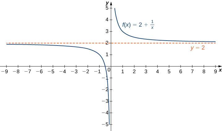
Figure 1. The function approaches the asymptote [latex]y=2[/latex] as [latex]x[/latex] approaches [latex]\pm \infty[/latex].

More generally, for any function [latex]f[/latex], we say the limit as [latex]x \to \infty[/latex] of [latex]f(x)[/latex] is [latex]L[/latex] if [latex]f(x)[/latex] becomes arbitrarily close to [latex]L[/latex] as long as [latex]x[/latex] is sufficiently large. In that case, we write [latex]\underset{x\to \infty}{\lim}f(x)=L[/latex]. Similarly, we say the limit as [latex]x\to −\infty[/latex] of [latex]f(x)[/latex] is [latex]L[/latex] if [latex]f(x)[/latex] becomes arbitrarily close to [latex]L[/latex] as long as [latex]x<0[/latex] and [latex]|x|[/latex] is sufficiently large. In that case, we write [latex]\underset{x\to −\infty }{\lim}f(x)=L[/latex]. We now look at the definition of a function having a limit at infinity.

If the values [latex]f(x)[/latex] are getting arbitrarily close to some finite value [latex]L[/latex] as [latex]x\to \infty[/latex] or [latex]x\to −\infty[/latex], the graph of [latex]f[/latex] approaches the line [latex]y=L[/latex]. In that case, the line [latex]y=L[/latex] is a horizontal asymptote of [latex]f[/latex] (Figure 2). For example, for the function [latex]f(x)=\frac{1}{x}[/latex], since [latex]\underset{x\to \infty }{\lim}f(x)=0[/latex], the line [latex]y=0[/latex] is a horizontal asymptote of [latex]f(x)=\frac{1}{x}[/latex].

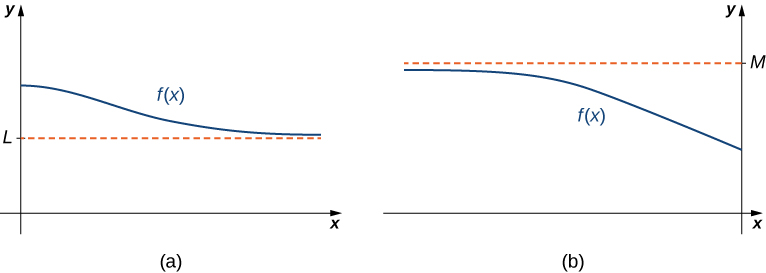
Figure 2. (a) As [latex]x\to \infty[/latex], the values of [latex]f[/latex] are getting arbitrarily close to [latex]L[/latex]. The line [latex]y=L[/latex] is a horizontal asymptote of [latex]f[/latex]. (b) As [latex]x\to −\infty[/latex], the values of [latex]f[/latex] are getting arbitrarily close to [latex]M[/latex]. The line [latex]y=M[/latex] is a horizontal asymptote of [latex]f[/latex].

A function cannot cross a vertical asymptote because the graph must approach infinity (or negative infinity) from at least one direction as [latex]x[/latex] approaches the vertical asymptote. However, a function may cross a horizontal asymptote. In fact, a function may cross a horizontal asymptote an unlimited number of times. For example, the function [latex]f(x)=\frac{ \cos x}{x}+1[/latex] shown in Figure 3 intersects the horizontal asymptote [latex]y=1[/latex] an infinite number of times as it oscillates around the asymptote with ever-decreasing amplitude.

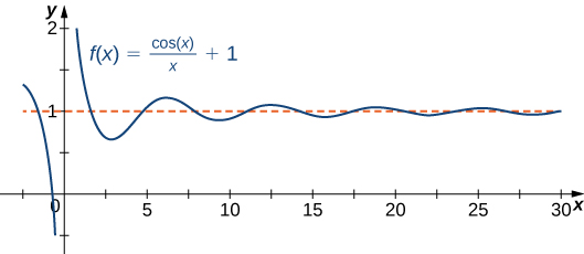
Figure 3. The graph of [latex]f(x)=\cos x/x+1[/latex] crosses its horizontal asymptote [latex]y=1[/latex] an infinite number of times.

The algebraic limit laws and squeeze theorem we introduced in Why It Matters: Limits also apply to limits at infinity. We illustrate how to use these laws to compute several limits at infinity.

Example: Computing Limits at Infinity

For each of the following functions [latex]f[/latex], evaluate [latex]\underset{x\to \infty }{\lim}f(x)[/latex] and [latex]\underset{x\to −\infty }{\lim}f(x)[/latex]. Determine the horizontal asymptote(s) for [latex]f[/latex].

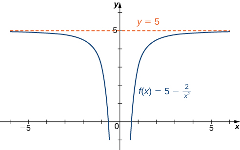
1. [latex]f(x)=5-\frac{2}{x^2}[/latex]
2. [latex]f(x)=\dfrac{\sin x}{x}[/latex]
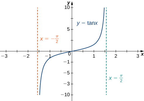
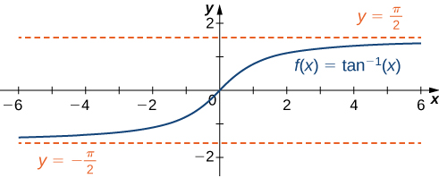
3. [latex]f(x)= \tan^{-1} (x)[/latex]

Show Solution

1. Using the algebraic limit laws, we have [latex]\underset{x\to \infty }{\lim}(5-\frac{2}{x^2})=\underset{x\to \infty }{\lim}5-2(\underset{x\to \infty }{\lim}\frac{1}{x})(\underset{x\to \infty }{\lim}\frac{1}{x})=5-2 \cdot 0=5[/latex]. Similarly, [latex]\underset{x\to -\infty }{\lim}f(x)=5[/latex]. Therefore, [latex]f(x)=5-\frac{2}{x^2}[/latex] has a horizontal asymptote of [latex]y=5[/latex] and [latex]f[/latex] approaches this horizontal asymptote as [latex]x\to \pm \infty[/latex] as shown in the following graph.
   

   Figure 4. This function approaches a horizontal asymptote as [latex]x\to \pm \infty[/latex].

2. Since [latex]-1\le \sin x\le 1[/latex] for all [latex]x[/latex], we have
   [latex]\frac{-1}{x}\le \frac{\sin x}{x}\le \frac{1}{x}[/latex]

   for all [latex]x \ne 0[/latex]. Also, since

   [latex]\underset{x\to \infty }{\lim}\frac{-1}{x}=0=\underset{x\to \infty }{\lim}\frac{1}{x}[/latex],

   we can apply the squeeze theorem to conclude that

   [latex]\underset{x\to \infty }{\lim}\frac{\sin x}{x}=0[/latex]

   Similarly,

   [latex]\underset{x\to −\infty}{\lim}\frac{\sin x}{x}=0[/latex]

    

   Thus, [latex]f(x)=\frac{\sin x}{x}[/latex] has a horizontal asymptote of [latex]y=0[/latex] and [latex]f(x)[/latex] approaches this horizontal asymptote as [latex]x\to \pm \infty[/latex] as shown in the following graph.

   

   Figure 5. This function crosses its horizontal asymptote multiple times.

3. To evaluate [latex]\underset{x\to \infty }{\lim} \tan^{-1} (x)[/latex] and [latex]\underset{x\to −\infty}{\lim} \tan^{-1} (x)[/latex], we first consider the graph of [latex]y= \tan (x)[/latex] over the interval [latex](−\pi /2,\pi /2)[/latex] as shown in the following graph.
   

   Figure 6. The graph of [latex] \tan x[/latex] has vertical asymptotes at [latex]x=\pm \frac{\pi }{2}[/latex]

Since

[latex]\underset{x\to (\pi/2)^-}{\lim} \tan x=\infty[/latex],

 

it follows that

[latex]\underset{x\to \infty }{\lim} \tan^{-1} (x)=\frac{\pi }{2}[/latex]

 

Similarly, since

[latex]\underset{x\to (\pi/2)^+}{\lim} \tan x=−\infty[/latex],

 

it follows that

[latex]\underset{x\to −\infty}{\lim} \tan^{-1} (x)=-\frac{\pi }{2}[/latex]

 

As a result, [latex]y=\frac{\pi }{2}[/latex] and [latex]y=-\frac{\pi }{2}[/latex] are horizontal asymptotes of [latex]f(x)= \tan^{-1} (x)[/latex] as shown in the following graph.

Figure 7. This function has two horizontal asymptotes.

Watch the following video to see the worked solution to Example: Computing Limits at Infinity.

Infinite Limits at Infinity

Sometimes the values of a function [latex]f[/latex] become arbitrarily large as [latex]x\to \infty[/latex] (or as [latex]x\to −\infty )[/latex]. In this case, we write [latex]\underset{x\to \infty }{\lim}f(x)=\infty[/latex] (or [latex]\underset{x\to −\infty }{\lim}f(x)=\infty )[/latex]. On the other hand, if the values of [latex]f[/latex] are negative but become arbitrarily large in magnitude as [latex]x\to \infty[/latex] (or as [latex]x\to −\infty )[/latex], we write [latex]\underset{x\to \infty }{\lim}f(x)=−\infty[/latex] (or [latex]\underset{x\to −\infty }{\lim}f(x)=−\infty )[/latex].

For example, consider the function [latex]f(x)=x^3[/latex]. As seen in the table below and Figure 8, as [latex]x\to \infty[/latex] the values [latex]f(x)[/latex] become arbitrarily large. Therefore, [latex]\underset{x\to \infty }{\lim}x^3=\infty[/latex]. On the other hand, as [latex]x\to −\infty[/latex], the values of [latex]f(x)=x^3[/latex] are negative but become arbitrarily large in magnitude. Consequently, [latex]\underset{x\to −\infty }{\lim}x^3=−\infty[/latex].

Values of a power function as [latex]x\to \pm \infty[/latex]

[latex]x[/latex]	10	20	50	100	1000
[latex]x^3[/latex]	1000	8000	125,000	1,000,000	1,000,000,000
[latex]x[/latex]	-10	-20	-50	-100	-1000
[latex]x^3[/latex]	-1000	-8000	-125,000	-1,000,000	-1,000,000,000

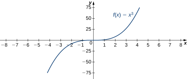
Figure 8. For this function, the functional values approach infinity as [latex]x\to \pm \infty[/latex].

Definition

---

(Informal) We say a function [latex]f[/latex] has an infinite limit at infinity and write

[latex]\underset{x\to \infty }{\lim}f(x)=\infty[/latex]

 

if [latex]f(x)[/latex] becomes arbitrarily large for [latex]x[/latex] sufficiently large. We say a function has a negative infinite limit at infinity and write

[latex]\underset{x\to \infty }{\lim}f(x)=−\infty[/latex]

 

if [latex]f(x)<0[/latex] and [latex]|f(x)|[/latex] becomes arbitrarily large for [latex]x[/latex] sufficiently large. Similarly, we can define infinite limits as [latex]x\to −\infty[/latex].

Formal Definitions

Earlier, we used the terms arbitrarily close, arbitrarily large, and sufficiently large to define limits at infinity informally. Although these terms provide accurate descriptions of limits at infinity, they are not precise mathematically. Here are more formal definitions of limits at infinity. We then look at how to use these definitions to prove results involving limits at infinity.

Definition

---

(Formal) We say a function [latex]f[/latex] has a limit at infinity, if there exists a real number [latex]L[/latex] such that for all [latex]\varepsilon >0[/latex], there exists [latex]N>0[/latex] such that

[latex]|f(x)-L|<\varepsilon[/latex]

 

for all [latex]x>N[/latex]. In that case, we write

[latex]\underset{x\to \infty }{\lim}f(x)=L[/latex]

 

(see Figure 9).

 

We say a function [latex]f[/latex] has a limit at negative infinity if there exists a real number [latex]L[/latex] such that for all [latex]\varepsilon >0[/latex], there exists [latex]N<0[/latex] such that

[latex]|f(x)-L|<\varepsilon[/latex]

 

for all [latex]x

[latex]\underset{x\to −\infty }{\lim}f(x)=L[/latex]

 

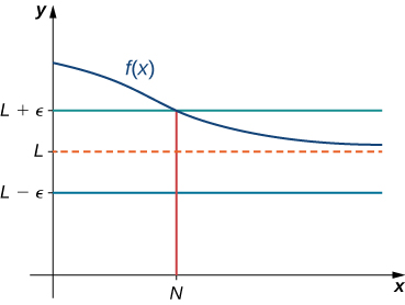
Figure 9. For a function with a limit at infinity, for all [latex]x>N[/latex], [latex]|f(x)-L|<\varepsilon [/latex].

Earlier in this section, we used graphical evidence and numerical evidence to conclude that [latex]\underset{x\to \infty }{\lim}\left(2+\frac{1}{x}\right)=2[/latex]. Here we use the formal definition of limit at infinity to prove this result rigorously.

Example: A Finite Limit at Infinity Example

Use the formal definition of limit at infinity to prove that [latex]\underset{x\to \infty }{\lim}\left(2+\frac{1}{x}\right)=2[/latex].

Show Solution

Let [latex]\varepsilon >0[/latex]. Let [latex]N=\frac{1}{\varepsilon }[/latex]. Therefore, for all [latex]x>N[/latex], we have

[latex]\left| 2+\dfrac{1}{x}-2 \right| =\left| \dfrac{1}{x} \right|=\dfrac{1}{x}<\dfrac{1}{N}=\varepsilon[/latex].

Watch the following video to see the worked solution to Example: A Finite Limit at Infinity Example.

We now turn our attention to a more precise definition for an infinite limit at infinity.

Definition

---

(Formal) We say a function [latex]f[/latex] has an infinite limit at infinity and write

[latex]\underset{x\to \infty }{\lim}f(x)=\infty[/latex]

 

if for all [latex]M>0[/latex], there exists an [latex]N>0[/latex] such that

[latex]f(x)>M[/latex]

 

for all [latex]x>N[/latex] (see Figure 10).

 

We say a function has a negative infinite limit at infinity and write

[latex]\underset{x\to \infty }{\lim}f(x)=−\infty[/latex]

 

if for all [latex]M<0[/latex], there exists an [latex]N>0[/latex] such that

[latex]f(x)

 

for all [latex]x>N[/latex].

Similarly we can define limits as [latex]x\to −\infty[/latex].

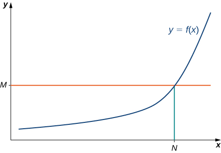
Figure 10. For a function with an infinite limit at infinity, for all [latex]x>N[/latex], [latex]f(x)>M[/latex].

Earlier, we used graphical evidence (Figure 8) and numerical evidence (the table beneath it) to conclude that [latex]\underset{x\to \infty }{\lim}x^3=\infty[/latex]. Here we use the formal definition of infinite limit at infinity to prove that result.

Example: An Infinite Limit at Infinity

Use the formal definition of infinite limit at infinity to prove that [latex]\underset{x\to \infty }{\lim}x^3=\infty[/latex].

Show Solution

Let [latex]M>0[/latex]. Let [latex]N=\sqrt[3]{M}[/latex]. Then, for all [latex]x>N[/latex], we have

[latex]x^3>N^3=(\sqrt[3]{M})^3=M[/latex].

 

Therefore, [latex]\underset{x\to \infty }{\lim}x^3=\infty[/latex].

Watch the following video to see the worked solution to Example: An Infinite Limit at Infinity.

Closed Captioning and Transcript Information for Video

For closed captioning, open the video on its original page by clicking the Youtube logo in the lower right-hand corner of the video display. In YouTube, the video will begin at the same starting point as this clip, but will continue playing until the very end.

You can view the transcript for this segmented clip of “4.6 Limits at Infinity and Asymptotes” here (opens in new window).

Try It

Use the formal definition of infinite limit at infinity to prove that [latex]\underset{x\to \infty }{\lim}3x^2=\infty[/latex].

Hint

Let [latex]N=\sqrt{\frac{M}{3}}[/latex].

Show Solution

Let [latex]M>0[/latex]. Let [latex]N=\sqrt{\frac{M}{3}}[/latex]. Then, for all [latex]x>N[/latex], we have

[latex]3x^2>3N^2=3(\sqrt{\frac{M}{3}})^2=\frac{3M}{3}=M[/latex]