1. State whether the given sums are equal or unequal.
- [latex]\underset{i=1}{\overset{10}{\Sigma}} i[/latex] and [latex]\underset{k=1}{\overset{10}{\Sigma}} k[/latex]
- [latex]\underset{i=1}{\overset{10}{\Sigma}} i[/latex] and [latex]\underset{i=6}{\overset{15}{\Sigma}} (i-5)[/latex]
- [latex]\underset{i=1}{\overset{10}{\Sigma}} i(i-1)[/latex] and [latex]\underset{j=0}{\overset{9}{\Sigma}} (j+1)j[/latex]
- [latex]\underset{i=1}{\overset{10}{\Sigma}} i(i-1)[/latex] and [latex]\underset{k=1}{\overset{10}{\Sigma}}(k^2-k)[/latex]
In the following exercises (2-3), use the rules for sums of powers of integers to compute the sums.
2. [latex]\displaystyle\sum_{i=5}^{10} i[/latex]
3. [latex]\displaystyle\sum_{i=5}^{10} i^2[/latex]
Suppose that [latex]\underset{i=1}{\overset{100}{\Sigma}} a_i=15[/latex] and [latex]\underset{i=1}{\overset{100}{\Sigma}} b_i=-12[/latex]. In the following exercises (4-7), compute the sums.
4. [latex]\displaystyle\sum_{i=1}^{100} (a_i+b_i)[/latex]
5. [latex]\displaystyle\sum_{i=1}^{100} (a_i-b_i)[/latex]
6. [latex]\displaystyle\sum_{i=1}^{100} (3a_i-4b_i)[/latex]
7. [latex]\displaystyle\sum_{i=1}^{100} (5a_i+4b_i)[/latex]
In the following exercises (8-11), use summation properties and formulas to rewrite and evaluate the sums.
8. [latex]\displaystyle\sum_{k=1}^{20} 100(k^2-5k+1)[/latex]
9. [latex]\displaystyle\sum_{j=1}^{50} (j^2-2j)[/latex]
10. [latex]\displaystyle\sum_{j=11}^{20} (j^2-10j)[/latex]
11. [latex]\displaystyle\sum_{k=1}^{25} [(2k)^2-100k][/latex]
Let [latex]L_n[/latex] denote the left-endpoint sum using [latex]n[/latex] subintervals and let [latex]R_n[/latex] denote the corresponding right-endpoint sum. In the following exercises (12-19), compute the indicated left and right sums for the given functions on the indicated interval.
12. [latex]L_4[/latex] for [latex]f(x)=\dfrac{1}{x-1}[/latex] on [latex][2,3][/latex]
13. [latex]R_4[/latex] for [latex]g(x)= \cos (\pi x)[/latex] on [latex][0,1][/latex]
14. [latex]L_6[/latex] for [latex]f(x)=\dfrac{1}{x(x-1)}[/latex] on [latex][2,5][/latex]
15. [latex]R_6[/latex] for [latex]f(x)=\dfrac{1}{x(x-1)}[/latex] on [latex][2,5][/latex]
16. [latex]R_4[/latex] for [latex]\dfrac{1}{x^2+1}[/latex] on [latex][-2,2][/latex]
17. [latex]L_4[/latex] for [latex]\dfrac{1}{x^2+1}[/latex] on [latex][-2,2][/latex]
18. [latex]R_4[/latex] for [latex]x^2-2x+1[/latex] on [latex][0,2][/latex]
19. [latex]L_8[/latex] for [latex]x^2-2x+1[/latex] on [latex][0,2][/latex]
20. Compute the left and right Riemann sums—[latex]L_4[/latex] and [latex]R_4[/latex], respectively—for [latex]f(x)=(2-|x|)[/latex] on [latex][-2,2][/latex]. Compute their average value and compare it with the area under the graph of [latex]f[/latex].
21. Compute the left and right Riemann sums—[latex]L_6[/latex] and [latex]R_6[/latex], respectively—for [latex]f(x)=(3-|3-x|)[/latex] on [latex][0,6][/latex]. Compute their average value and compare it with the area under the graph of [latex]f[/latex].
22. Compute the left and right Riemann sums—[latex]L_4[/latex] and [latex]R_4[/latex], respectively—for [latex]f(x)=\sqrt{4-x^2}[/latex] on [latex][-2,2][/latex] and compare their values.
23. Compute the left and right Riemann sums—[latex]L_6[/latex] and [latex]R_6[/latex], respectively—for [latex]f(x)=\sqrt{9-(x-3)^2}[/latex] on [latex][0,6][/latex] and compare their values.
Express the following endpoint sums in sigma notation but do not evaluate them (24-27).
24. [latex]L_{30}[/latex] for [latex]f(x)=x^2[/latex] on [latex][1,2][/latex]
25. [latex]L_{10}[/latex] for [latex]f(x)=\sqrt{4-x^2}[/latex] on [latex][-2,2][/latex]
26. [latex]R_{20}[/latex] for [latex]f(x)= \sin x[/latex] on [latex][0,\pi][/latex]
27. [latex]R_{100}[/latex] for [latex]\ln x[/latex] on [latex][1,e][/latex]
In the following exercises (28-33), graph the function then use a calculator or a computer program to evaluate the following left and right endpoint sums. Is the area under the curve between the left and right endpoint sums?
28. [T] [latex]L_{100}[/latex] and [latex]R_{100}[/latex] for [latex]y=x^2-3x+1[/latex] on the interval [latex][-1,1][/latex]
29. [T] [latex]L_{100}[/latex] and [latex]R_{100}[/latex] for [latex]y=x^2[/latex] on the interval [latex][0,1][/latex]
![A graph of the given function on the interval [0, 1]. It is set up for a left endpoint approximation and is an underestimate because the function is increasing. Ten rectangles are shown for visual clarity, but this behavior persists for more rectangles.](https://s3-us-west-2.amazonaws.com/courses-images/wp-content/uploads/sites/2332/2018/01/11203930/CNX_Calc_Figure_05_01_207.jpg)
30. [T] [latex]L_{50}[/latex] and [latex]R_{50}[/latex] for [latex]y=\dfrac{x+1}{x^2-1}[/latex] on the interval [latex][2,4][/latex]
31. [T] [latex]L_{100}[/latex] and [latex]R_{100}[/latex] for [latex]y=x^3[/latex] on the interval [latex][-1,1][/latex]
![A graph of the given function over [-1,1] set up for a left endpoint approximation. It is an underestimate since the function is increasing. Ten rectangles are shown for visual clarity, but this behavior persists for more rectangles.](https://s3-us-west-2.amazonaws.com/courses-images/wp-content/uploads/sites/2332/2018/01/11203933/CNX_Calc_Figure_05_01_209.jpg)
32. [T] [latex]L_{50}[/latex] and [latex]R_{50}[/latex] for [latex]y= \tan x[/latex] on the interval [latex]\left[0,\frac{\pi}{4}\right][/latex]
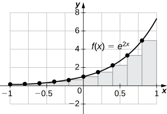
33. [T] [latex]L_{100}[/latex] and [latex]R_{100}[/latex] for [latex]y=e^{2x}[/latex] on the interval [latex][-1,1][/latex]
34. Let [latex]t_j[/latex] denote the time that it took Tejay van Garteren to ride the [latex]j[/latex]th stage of the Tour de France in 2014. If there were a total of 21 stages, interpret [latex]\displaystyle\sum_{j=1}^{21} t_j[/latex].
35. Let [latex]r_j[/latex] denote the total rainfall in Portland on the [latex]j[/latex]th day of the year in 2009. Interpret [latex]\displaystyle\sum_{j=1}^{31} r_j[/latex].
36. Let [latex]d_j[/latex] denote the hours of daylight and [latex]\delta_j[/latex] denote the increase in the hours of daylight from day [latex]j-1[/latex] to day [latex]j[/latex] in Fargo, North Dakota, on the [latex]j[/latex]th day of the year. Interpret [latex]d_1+\underset{j=2}{\overset{365}{\Sigma}} \delta_j[/latex].
37. To help get in shape, Joe gets a new pair of running shoes. If Joe runs 1 mi each day in week 1 and adds [latex]\frac{1}{10}[/latex] mi to his daily routine each week, what is the total mileage on Joe’s shoes after 25 weeks?
38. The following table gives approximate values of the average annual atmospheric rate of increase in carbon dioxide (CO2) each decade since 1960, in parts per million (ppm). Estimate the total increase in atmospheric CO2 between 1964 and 2013.
| Decade | Ppm/y |
|---|---|
| 1964–1973 | 1.07 |
| 1974–1983 | 1.34 |
| 1984–1993 | 1.40 |
| 1994–2003 | 1.87 |
| 2004–2013 | 2.07 |
39. The following table gives the approximate increase in sea level in inches over 20 years starting in the given year. Estimate the net change in mean sea level from 1870 to 2010.
| Starting Year | 20-Year Change |
|---|---|
| 1870 | 0.3 |
| 1890 | 1.5 |
| 1910 | 0.2 |
| 1930 | 2.8 |
| 1950 | 0.7 |
| 1970 | 1.1 |
| 1990 | 1.5 |
40. The following table gives the approximate increase in dollars in the average price of a gallon of gas per decade since 1950. If the average price of a gallon of gas in 2010 was $2.60, what was the average price of a gallon of gas in 1950?
| Starting Year | 10-Year Change |
|---|---|
| 1950 | 0.03 |
| 1960 | 0.05 |
| 1970 | 0.86 |
| 1980 | −0.03 |
| 1990 | 0.29 |
| 2000 | 1.12 |
41. The following table gives the percent growth of the U.S. population beginning in July of the year indicated. If the U.S. population was 281,421,906 in July 2000, estimate the U.S. population in July 2010.
| Year | % Change/Year |
|---|---|
| 2000 | 1.12 |
| 2001 | 0.99 |
| 2002 | 0.93 |
| 2003 | 0.86 |
| 2004 | 0.93 |
| 2005 | 0.93 |
| 2006 | 0.97 |
| 2007 | 0.96 |
| 2008 | 0.95 |
| 2009 | 0.88 |
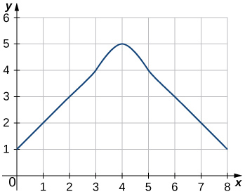
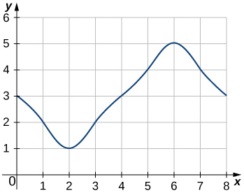
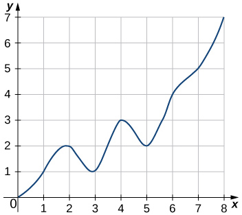
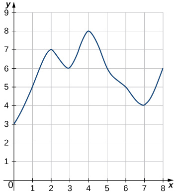
In the following exercises (42-45), estimate the areas under the curves by computing the left Riemann sums, [latex]L_8[/latex].
46. [T] Use a computer algebra system to compute the Riemann sum, [latex]L_N[/latex], for [latex]N=10,30,50[/latex] for [latex]f(x)=\sqrt{1-x^2}[/latex] on [latex][-1,1][/latex].
47. [T] Use a computer algebra system to compute the Riemann sum, [latex]L_N[/latex], for [latex]N=10,30,50[/latex] for [latex]f(x)=\dfrac{1}{\sqrt{1+x^2}}[/latex] on [latex][-1,1][/latex].
48. [T] Use a computer algebra system to compute the Riemann sum, [latex]L_N[/latex], for [latex]N=10,30,50[/latex] for [latex]f(x)= \sin^2 x[/latex] on [latex][0,2\pi][/latex]. Compare these estimates with [latex]\pi[/latex].
In the following exercises (49-50), use a calculator or a computer program to evaluate the endpoint sums [latex]R_N[/latex] and [latex]L_N[/latex] for [latex]N=1,10,100[/latex]. How do these estimates compare with the exact answers, which you can find via geometry?
49. [T] [latex]y= \cos (\pi x)[/latex] on the interval [latex][0,1][/latex]
50. [T] [latex]y=3x+2[/latex] on the interval [latex][3,5][/latex]
In the following exercises (51-52), use a calculator or a computer program to evaluate the endpoint sums [latex]R_N[/latex] and [latex]L_N[/latex] for [latex]N=1,10,100[/latex].
51. [T] [latex]y=x^4-5x^2+4[/latex] on the interval [latex][-2,2][/latex], which has an exact area of [latex]\frac{32}{15}[/latex]
52. [T] [latex]y=\ln x[/latex] on the interval [latex][1,2][/latex], which has an exact area of [latex]2\ln (2)-1[/latex]
53. Explain why, if [latex]f(a)\ge 0[/latex] and [latex]f[/latex] is increasing on [latex][a,b][/latex], that the left endpoint estimate is a lower bound for the area below the graph of [latex]f[/latex] on [latex][a,b][/latex].
54. Explain why, if [latex]f(b)\ge 0[/latex] and [latex]f[/latex] is decreasing on [latex][a,b][/latex], that the left endpoint estimate is an upper bound for the area below the graph of [latex]f[/latex] on [latex][a,b][/latex].
55. Show that, in general, [latex]R_N-L_N=(b-a) \times \frac{f(b)-f(a)}{N}[/latex].
56. Explain why, if [latex]f[/latex] is increasing on [latex][a,b][/latex], the error between either [latex]L_N[/latex] or [latex]R_N[/latex] and the area [latex]A[/latex] below the graph of [latex]f[/latex] is at most [latex](b-a)\frac{f(b)-f(a)}{N}[/latex].
57. For each of the three graphs:
- Obtain a lower bound [latex]L(A)[/latex] for the area enclosed by the curve by adding the areas of the squares enclosed completely by the curve.
- Obtain an upper bound [latex]U(A)[/latex] for the area by adding to [latex]L(A)[/latex] the areas [latex]B(A)[/latex] of the squares enclosed partially by the curve.
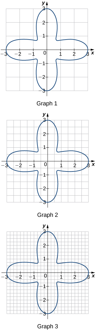
58. In the previous exercise, explain why [latex]L(A)[/latex] gets no smaller while [latex]U(A)[/latex] gets no larger as the squares are subdivided into four boxes of equal area.
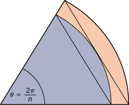
59. A unit circle is made up of [latex]n[/latex] wedges equivalent to the inner wedge in the figure. The base of the inner triangle is 1 unit and its height is [latex]\sin \left(\frac{\pi }{n}\right)[/latex]. The base of the outer triangle is [latex]B= \cos \left(\frac{\pi }{n}\right)+ \sin \left(\frac{\pi }{n}\right) \tan \left(\frac{\pi }{n}\right)[/latex] and the height is [latex]H=B \sin \left(\frac{2\pi }{n}\right)[/latex]. Use this information to argue that the area of a unit circle is equal to [latex]\pi[/latex].
Candela Citations
- Calculus Volume 1. Authored by: Gilbert Strang, Edwin (Jed) Herman. Provided by: OpenStax. Located at: https://openstax.org/details/books/calculus-volume-1. License: CC BY-NC-SA: Attribution-NonCommercial-ShareAlike. License Terms: Access for free at https://openstax.org/books/calculus-volume-1/pages/1-introduction
