For the following exercises (1-10), use the definition of a derivative to find the slope of the secant line between the values [latex]x_1[/latex] and [latex]x_2[/latex] for each function [latex]y=f(x)[/latex].
1. [latex]f(x)=4x+7; \,\,\, x_1=2, \,\,\, x_2=5[/latex]
2. [latex]f(x)=8x-3; \,\,\, x_1=-1, \,\,\, x_2=3[/latex]
3. [latex]f(x)=x^2+2x+1; \,\,\, x_1=3, \,\,\, x_2=3.5[/latex]
4. [latex]f(x)=\text{−}{x}^{2}+x+2;{x}_{1}=0.5,{x}_{2}=1.5[/latex]
5. [latex]f(x)=\dfrac{4}{3x-1}; \,\,\, x_1=1, \,\,\, x_2=3[/latex]
6. [latex]f(x)=\dfrac{x-7}{2x+1}; \,\,\, x_1=0, \,\,\, x_2=2[/latex]
7. [latex]f(x)=\sqrt{x}; \,\,\, x_1=1, \,\,\, x_2=16[/latex]
8. [latex]f(x)=\sqrt{x-9}; \,\,\, x_1=10, \,\,\, x_2=13[/latex]
9. [latex]f(x)=x^{\frac{1}{3}}+1; \,\,\, x_1=0, \,\,\, x_2=8[/latex]
10. [latex]f(x)=6x^{\frac{2}{3}}+2x^{\frac{1}{3}}; \,\,\, x_1=1, \,\,\, x_2=27[/latex]
For the following functions (11-20),
- Use [latex]m_{\tan}=\underset{h\to 0}{\lim}\dfrac{f(a+h)-f(a)}{h}[/latex] to find the slope of the tangent line [latex]m_{\tan}=f^{\prime}(a)[/latex], and
- find the equation of the tangent line to [latex]f[/latex] at [latex]x=a[/latex].
11. [latex]f(x)=3-4x, \,\,\, a=2[/latex]
12. [latex]f(x)=\dfrac{x}{5}+6, \,\,\, a=-1[/latex]
13. [latex]f(x)=x^2+x, \,\,\, a=1[/latex]
14. [latex]f(x)=1-x-x^2, \,\,\, a=0[/latex]
15. [latex]f(x)=\dfrac{7}{x}, \,\,\, a=3[/latex]
16. [latex]f(x)=\sqrt{x+8}, \,\,\, a=1[/latex]
17. [latex]f(x)=2-3x^2, \,\,\, a=-2[/latex]
18. [latex]f(x)=\dfrac{-3}{x-1}, \,\,\, a=4[/latex]
19. [latex]f(x)=\dfrac{2}{x+3}, \,\,\, a=-4[/latex]
20. [latex]f(x)=\dfrac{3}{x^2}, \,\,\, a=3[/latex]
For the following functions [latex]y=f(x)[/latex] (21-30), find [latex]f^{\prime}(a)[/latex] using [latex]f^{\prime}(a)=\underset{x\to a}{\lim}\dfrac{f(x)-f(a)}{x-a}[/latex].
21. [latex]f(x)=5x+4, \,\,\, a=-1[/latex]
22. [latex]f(x)=-7x+1, \,\,\, a=3[/latex]
23. [latex]f(x)=x^2+9x, \,\,\, a=2[/latex]
24. [latex]f(x)=3x^2-x+2, \,\,\, a=1[/latex]
25. [latex]f(x)=\sqrt{x}, \,\,\, a=4[/latex]
26. [latex]f(x)=\sqrt{x-2}, \,\,\, a=6[/latex]
27. [latex]f(x)=\dfrac{1}{x}, \,\,\, a=2[/latex]
28. [latex]f(x)=\dfrac{1}{x-3}, \,\,\, a=-1[/latex]
29. [latex]f(x)=\dfrac{1}{x^3}, \,\,\, a=1[/latex]
30. [latex]f(x)=\dfrac{1}{\sqrt{x}}, \,\,\, a=4[/latex]
For the following exercises (31-34), given the function [latex]y=f(x)[/latex],
- find the slope of the secant line [latex]PQ[/latex] for each point [latex]Q(x,f(x))[/latex] with [latex]x[/latex] value given in the table.
- Use the answers from a. to estimate the value of the slope of the tangent line at [latex]P[/latex].
- Use the answer from b. to find the equation of the tangent line to [latex]f[/latex] at point [latex]P[/latex].
31. [T] [latex]f(x)=x^2+3x+4, \,\,\, P(1,8)[/latex] (Round to 6 decimal places.)
| [latex]x[/latex] | Slope [latex]m_{PQ}[/latex] | [latex]x[/latex] | Slope [latex]m_{PQ}[/latex] |
|---|---|---|---|
| 1.1 | (i) | 0.9 | (vii) |
| 1.01 | (ii) | 0.99 | (viii) |
| 1.001 | (iii) | 0.999 | (ix) |
| 1.0001 | (iv) | 0.9999 | (x) |
| 1.00001 | (v) | 0.99999 | (xi) |
| 1.000001 | (vi) | 0.999999 | (xii) |
32. [T] [latex]f(x)=\dfrac{x+1}{x^2-1}, \,\,\, P(0,-1)[/latex]
| [latex]x[/latex] | Slope [latex]m_{PQ}[/latex] | [latex]x[/latex] | Slope [latex]m_{PQ}[/latex] |
|---|---|---|---|
| 0.1 | (i) | -0.1 | (vii) |
| 0.01 | (ii) | -0.01 | (viii) |
| 0.001 | (iii) | -0.001 | (ix) |
| 0.0001 | (iv) | -0.0001 | (x) |
| 0.00001 | (v) | -0.00001 | (xi) |
| 0.000001 | (vi) | -0.000001 | (xii) |
33. [T] [latex]f(x)=10e^{0.5x}, \,\,\, P(0,10)[/latex] (Round to 4 decimal places.)
| [latex]x[/latex] | Slope [latex]m_{PQ}[/latex] |
|---|---|
| -0.1 | (i) |
| -0.01 | (ii) |
| -0.001 | (iii) |
| -0.0001 | (iv) |
| -0.00001 | (v) |
| −0.000001 | (vi) |
34. [T] [latex]f(x)= \tan (x), \,\,\, P(\pi,0)[/latex]
| [latex]x[/latex] | Slope [latex]m_{PQ}[/latex] |
|---|---|
| 3.1 | (i) |
| 3.14 | (ii) |
| 3.141 | (iii) |
| 3.1415 | (iv) |
| 3.14159 | (v) |
| 3.141592 | (vi) |
For the following position functions [latex]y=s(t)[/latex], an object is moving along a straight line, where [latex]t[/latex] is in seconds and [latex]s[/latex] is in meters. Find
- the simplified expression for the average velocity from [latex]t=2[/latex] to [latex]t=2+h[/latex];
- the average velocity between [latex]t=2[/latex] and [latex]t=2+h[/latex], where (i) [latex]h=0.1[/latex], (ii) [latex]h=0.01[/latex], (iii) [latex]h=0.001[/latex], and (iv) [latex]h=0.0001[/latex]; and
- use the answer from a. to estimate the instantaneous velocity at [latex]t=2[/latex] seconds.
35. [T] [latex]s(t)=\frac{1}{3}t+5[/latex]
36. [T] [latex]s(t)=t^2-2t[/latex]
37. [T] [latex]s(t)=2t^3+3[/latex]
38. [T] [latex]s(t)=\dfrac{16}{t^2}-\dfrac{4}{t}[/latex]
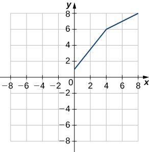
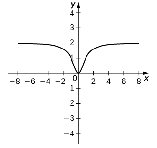
39. Use the following graph to evaluate a. [latex]f^{\prime}(1)[/latex] and b. [latex]f^{\prime}(6)[/latex].
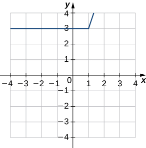
40. Use the following graph to evaluate a. [latex]f^{\prime}(-3)[/latex] and b. [latex]f^{\prime}(1.5)[/latex].
For the following exercises, use the limit definition of derivative to show that the derivative does not exist at [latex]x=a[/latex] for each of the given functions.
41. [latex]f(x)=x^{\frac{1}{3}}, \, x=0[/latex]
42. [latex]f(x)=x^{\frac{2}{3}}, \, x=0[/latex]
43. [latex]f(x)=\begin{cases} 1 & \text{ if } \, x<1 \\ x & \text{ if } \, x \ge 1 \end{cases}, \, x=1[/latex]
44. [latex]f(x)=\dfrac{|x|}{x}, \, x=0[/latex]
45. [T] The position in feet of a race car along a straight track after [latex]t[/latex] seconds is modeled by the function [latex]s(t)=8t^2-\frac{1}{16}t^3[/latex].
- Find the average velocity of the vehicle over the following time intervals to four decimal places:
- [4, 4.1]
- [4, 4.01]
- [4, 4.001]
- [4, 4.0001]
- Use a. to draw a conclusion about the instantaneous velocity of the vehicle at [latex]t=4[/latex] seconds.
46. [T] The distance in feet that a ball rolls down an incline is modeled by the function [latex]s(t)=14t^2[/latex], where [latex]t[/latex] is seconds after the ball begins rolling.
- Find the average velocity of the ball over the following time intervals:
- [5, 5.1]
- [5, 5.01]
- [5, 5.001]
- [5, 5.0001]
- Use the answers from a. to draw a conclusion about the instantaneous velocity of the ball at [latex]t=5[/latex] seconds.
47. Two vehicles start out traveling side by side along a straight road. Their position functions, shown in the following graph, are given by [latex]s=f(t)[/latex] and [latex]s=g(t)[/latex], where [latex]s[/latex] is measured in feet and [latex]t[/latex] is measured in seconds.
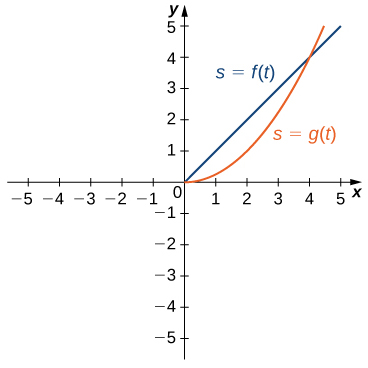
- Which vehicle has traveled farther at [latex]t=2[/latex] seconds?
- What is the approximate velocity of each vehicle at [latex]t=3[/latex] seconds?
- Which vehicle is traveling faster at [latex]t=4[/latex] seconds?
- What is true about the positions of the vehicles at [latex]t=4[/latex] seconds?
48. [T] The total cost [latex]C(x)[/latex], in hundreds of dollars, to produce [latex]x[/latex] jars of mayonnaise is given by [latex]C(x)=0.000003x^3+4x+300[/latex].
- Calculate the average cost per jar over the following intervals:
- [100, 100.1]
- [100, 100.01]
- [100, 100.001]
- [100, 100.0001]
- Use the answers from a. to estimate the average cost to produce 100 jars of mayonnaise.
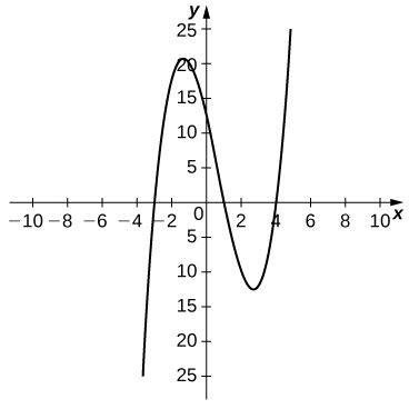
49. [T] For the function [latex]f(x)=x^3-2x^2-11x+12[/latex], do the following.
- Use a graphing calculator to graph [latex]f[/latex] in an appropriate viewing window.
- Use the ZOOM feature on the calculator to approximate the two values of [latex]x=a[/latex] for which [latex]m_{\tan}=f^{\prime}(a)=0[/latex].
50. [T] For the function [latex]f(x)=\dfrac{x}{1+x^2}[/latex], do the following.
- Use a graphing calculator to graph [latex]f[/latex] in an appropriate viewing window.
- Use the ZOOM feature on the calculator to approximate the values of [latex]x=a[/latex] for which [latex]m_{\tan}=f^{\prime}(a)=0[/latex].
51. Suppose that [latex]N(x)[/latex] computes the number of gallons of gas used by a vehicle traveling [latex]x[/latex] miles. Suppose the vehicle gets 30 mpg.
- Find a mathematical expression for [latex]N(x)[/latex].
- What is [latex]N(100)[/latex]? Explain the physical meaning.
- What is [latex]N^{\prime}(100)[/latex]? Explain the physical meaning.
52. [T] For the function [latex]f(x)=x^4-5x^2+4[/latex], do the following.
- Use a graphing calculator to graph [latex]f[/latex] in an appropriate viewing window.
- Use the [latex]\text{nDeriv}[/latex] function, which numerically finds the derivative, on a graphing calculator to estimate [latex]f^{\prime}(-2), \, f^{\prime}(-0.5), \, f^{\prime}(1.7)[/latex], and [latex]f^{\prime}(2.718)[/latex].
53. [T] For the function [latex]f(x)=\dfrac{x^2}{x^2+1}[/latex], do the following.
- Use a graphing calculator to graph [latex]f[/latex] in an appropriate viewing window.
- Use the [latex]\text{nDeriv}[/latex] function on a graphing calculator to find [latex]f^{\prime}(-4), \, f^{\prime}(-2), \, f^{\prime}(2)[/latex], and [latex]f^{\prime}(4)[/latex].
Candela Citations
- Calculus Volume 1. Authored by: Gilbert Strang, Edwin (Jed) Herman. Provided by: OpenStax. Located at: https://openstax.org/details/books/calculus-volume-1. License: CC BY-NC-SA: Attribution-NonCommercial-ShareAlike. License Terms: Access for free at https://openstax.org/books/calculus-volume-1/pages/1-introduction
