1. If [latex]c[/latex] is a critical point of [latex]f(x)[/latex], when is there no local maximum or minimum at [latex]c[/latex]? Explain.
2. For the function [latex]y=x^3[/latex], is [latex]x=0[/latex] both an inflection point and a local maximum/minimum?
3. For the function [latex]y=x^3[/latex], is [latex]x=0[/latex] an inflection point?
4. Is it possible for a point [latex]c[/latex] to be both an inflection point and a local extrema of a twice differentiable function?
5. Why do you need continuity for the first derivative test? Come up with an example.
6. Explain whether a concave-down function has to cross [latex]y=0[/latex] for some value of [latex]x[/latex].
7. Explain whether a polynomial of degree 2 can have an inflection point.
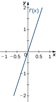
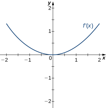
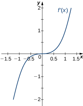
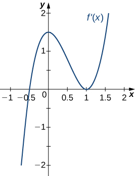
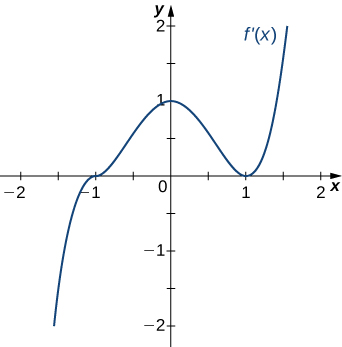
For the following exercises (8-12), analyze the graphs of [latex]f^{\prime}[/latex], then list all intervals where [latex]f[/latex] is increasing or decreasing.
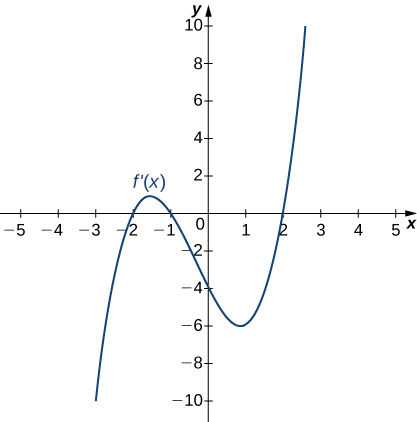
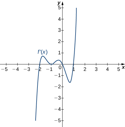
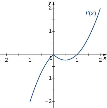
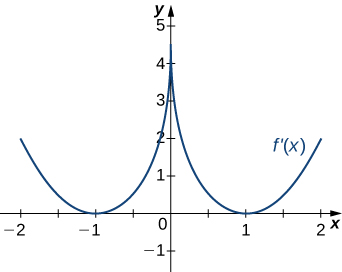
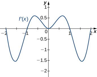
For the following exercises (13-17), analyze the graphs of [latex]f^{\prime}[/latex], then list
- all intervals where [latex]f[/latex] is increasing and decreasing and
- where the minima and maxima are located.
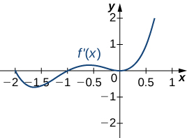
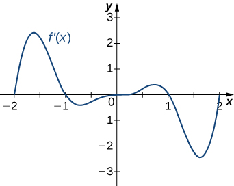
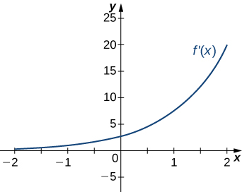
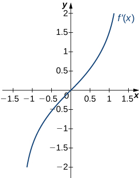
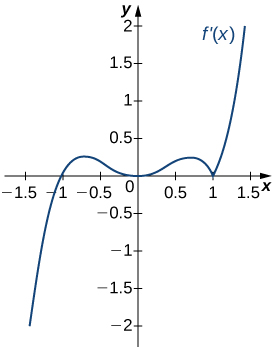
For the following exercises (18-22), analyze the graphs of [latex]f^{\prime}[/latex], then list all inflection points and intervals [latex]f[/latex] that are concave up and concave down.
For the following exercises (23-27), draw a graph that satisfies the given specifications for the domain [latex]x=[-3,3][/latex]. The function does not have to be continuous or differentiable.
23. [latex]f(x)>0, \, f^{\prime}(x)>0[/latex] over [latex]x>1, \, -3
24. [latex]f^{\prime}(x)>0[/latex] over [latex]x>2, \, -3
25. [latex]f^{\prime \prime}(x)<0[/latex] over [latex]-1
26. There is a local maximum at [latex]x=2[/latex], local minimum at [latex]x=1[/latex], and the graph is neither concave up nor concave down.
27. There are local maxima at [latex]x=\pm 1[/latex], the function is concave up for all [latex]x[/latex], and the function remains positive for all [latex]x[/latex].
For the following exercise, determine a. intervals where [latex]f[/latex] is concave up or concave down, and b. the inflection points of [latex]f[/latex].
30. [latex]f(x)=x^3-4x^2+x+2[/latex]
For the following exercises (31-37), determine
- intervals where [latex]f[/latex] is increasing or decreasing,
- local minima and maxima of [latex]f[/latex],
- intervals where [latex]f[/latex] is concave up and concave down, and
- the inflection points of [latex]f[/latex].
31. [latex]f(x)=x^2-6x[/latex]
32. [latex]f(x)=x^3-6x^2[/latex]
33. [latex]f(x)=x^4-6x^3[/latex]
34. [latex]f(x)=x^{11}-6x^{10}[/latex]
35. [latex]f(x)=x+x^2-x^3[/latex]
36. [latex]f(x)=x^2+x+1[/latex]
37. [latex]f(x)=x^3+x^4[/latex]
For the following exercises (38-47), determine
- intervals where [latex]f[/latex] is increasing or decreasing,
- local minima and maxima of [latex]f[/latex],
- intervals where [latex]f[/latex] is concave up and concave down, and
- the inflection points of [latex]f[/latex]. Sketch the curve, then use a calculator to compare your answer. If you cannot determine the exact answer analytically, use a calculator.
38. [T] [latex]f(x)= \sin (\pi x)- \cos (\pi x)[/latex] over [latex]x=[-1,1][/latex]
39. [T] [latex]f(x)=x + \sin (2x)[/latex] over [latex]x=\left[-\frac{\pi }{2},\frac{\pi }{2}\right][/latex]
40. [T] [latex]f(x)= \sin x+ \tan x[/latex] over [latex]\left(-\frac{\pi }{2},\frac{\pi }{2}\right)[/latex]
41. [T] [latex]f(x)=(x-2)^2 (x-4)^2[/latex]
42. [T] [latex]f(x)=\dfrac{1}{1-x}, \, x \ne 1[/latex]
43. [T] [latex]f(x)=\dfrac{\sin x}{x}[/latex] over [latex]x=[-2\pi ,0) \cup (0,2\pi][/latex]
44. [latex]f(x)= \sin x e^x[/latex] over [latex]x=[−\pi ,\pi][/latex]
45. [latex]f(x)=\ln x \sqrt{x}, \, x>0[/latex]
46. [latex]f(x)=\frac{1}{4}\sqrt{x}+\frac{1}{x}, \, x>0[/latex]
47. [latex]f(x)=\dfrac{e^x}{x}, \, x\ne 0[/latex]
For the following exercises (48-52), interpret the sentences in terms of [latex]f, \, f^{\prime}[/latex], and [latex]f^{\prime \prime}[/latex].
48. The population is growing more slowly. Here [latex]f[/latex] is the population.
49. A bike accelerates faster, but a car goes faster. Here [latex]f[/latex] represents the Bike’s position minus the Car’s position.
50. The airplane lands smoothly. Here [latex]f[/latex] is the plane’s altitude.
51. Stock prices are at their peak. Here [latex]f[/latex] is the stock price.
52. The economy is picking up speed. Here [latex]f[/latex] is a measure of the economy, such as GDP.
For the following exercises (53-57), consider a third-degree polynomial [latex]f(x)[/latex], which has the properties [latex]f^{\prime}(1)=0, \, f^{\prime}(3)=0[/latex]. Determine whether the following statements are true or false. Justify your answer.
53. [latex]f(x)=0[/latex] for some [latex]1 \le x \le 3[/latex]
54. [latex]f^{\prime \prime}(x)=0[/latex] for some [latex]1 \le x \le 3[/latex]
55. There is no absolute maximum at [latex]x=3[/latex]
56. If [latex]f(x)[/latex] has three roots, then it has 1 inflection point.
57. If [latex]f(x)[/latex] has one inflection point, then it has three real roots.
Candela Citations
- Calculus Volume 1. Authored by: Gilbert Strang, Edwin (Jed) Herman. Provided by: OpenStax. Located at: https://openstax.org/details/books/calculus-volume-1. License: CC BY-NC-SA: Attribution-NonCommercial-ShareAlike. License Terms: Access for free at https://openstax.org/books/calculus-volume-1/pages/1-introduction
