We now demonstrate how to use the epsilon-delta definition of a limit to construct a rigorous proof of one of the limit laws. The triangle inequality is used at a key point of the proof, so we first review this key property of absolute value.

Proof

We prove the following limit law: If [latex]\underset{x\to a}{\lim}f(x)=L[/latex] and [latex]\underset{x\to a}{\lim}g(x)=M[/latex], then [latex]\underset{x\to a}{\lim}(f(x)+g(x))=L+M[/latex].

Let [latex]\varepsilon >0[/latex].

Choose [latex]\delta_1>0[/latex] so that if [latex]0<|x-a|<\delta_1[/latex], then [latex]|f(x)-L|<\varepsilon/2[/latex].

Choose [latex]\delta_2>0[/latex] so that if [latex]0<|x-a|<\delta_2[/latex], then [latex]|g(x)-M|<\varepsilon/2[/latex].

Choose [latex]\delta =\text{min}\{\delta_1,\delta_2\}[/latex].

Assume [latex]0<|x-a|<\delta[/latex].

Thus,

[latex]0<|x-a|<\delta_1[/latex] and [latex]0<|x-a|<\delta_2[/latex]

Hence,

[latex]\begin{array}{ll} |(f(x)+g(x))-(L+M)| & =|(f(x)-L)+(g(x)-M)| \\ & \le |f(x)-L|+|g(x)-M| \\ & <\dfrac{\varepsilon}{2}+\dfrac{\varepsilon}{2}=\varepsilon \end{array}[/latex]

[latex]\blacksquare[/latex]

 

We now explore what it means for a limit not to exist. The limit [latex]\underset{x\to a}{\lim}f(x)[/latex] does not exist if there is no real number [latex]L[/latex] for which [latex]\underset{x\to a}{\lim}f(x)=L[/latex]. Thus, for all real numbers [latex]L[/latex], [latex]\underset{x\to a}{\lim}f(x)\ne L[/latex]. To understand what this means, we look at each part of the definition of [latex]\underset{x\to a}{\lim}f(x)=L[/latex] together with its opposite. A translation of the definition is given in the table below.

Translation of the Definition of [latex]\underset{x\to a}{\lim}f(x)=L[/latex] and its Opposite

Definition	Opposite
1. For every [latex]\varepsilon >0[/latex],	1. There exists [latex]\varepsilon >0[/latex] so that
2. there exists a [latex]\delta >0[/latex] so that	2. for every [latex]\delta >0[/latex],
3. if [latex]0<|x-a|<\delta[/latex], then [latex]|f(x)-L|<\varepsilon[/latex].	3. There is an [latex]x[/latex] satisfying [latex]0<|x-a|<\delta [/latex] so that [latex]|f(x)-L|\ge \varepsilon[/latex].

Finally, we may state what it means for a limit not to exist. The limit [latex]\underset{x\to a}{\lim}f(x)[/latex] does not exist if for every real number [latex]L[/latex], there exists a real number [latex]\varepsilon >0[/latex] so that for all [latex]\delta >0[/latex], there is an [latex]x[/latex] satisfying [latex]0<|x-a|<\delta[/latex], so that [latex]|f(x)-L|\ge \varepsilon[/latex]. Let’s apply this in the example to show that a limit does not exist.

Example: Showing That a Limit Does Not Exist

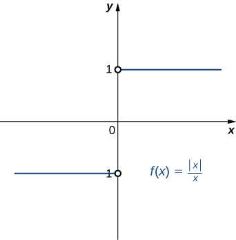
Show that [latex]\underset{x\to 0}{\lim}\dfrac{|x|}{x}[/latex] does not exist. The graph of [latex]f(x)=\dfrac{|x|}{x}[/latex] is shown here:

Figure 4.

Show Solution

Suppose that [latex]L[/latex] is a candidate for a limit. Choose [latex]\varepsilon =\frac{1}{2}[/latex].

Let [latex]\delta >0[/latex]. Either [latex]L\ge 0[/latex] or [latex]L<0[/latex]. If [latex]L\ge 0[/latex], then let [latex]x=-\delta/2[/latex]. Thus,

[latex]|x-0|=|-\frac{\delta}{2}-0|=\frac{\delta}{2}<\delta [/latex]

and

[latex]|\frac{|-\frac{\delta}{2}|}{-\frac{\delta}{2}}-L|=|-1-L|=L+1\ge 1>\frac{1}{2}=\varepsilon[/latex]

On the other hand, if [latex]L<0[/latex], then let [latex]x=\delta/2[/latex]. Thus,

[latex]|x-0|=|\frac{\delta}{2}-0|=\frac{\delta}{2}<\delta [/latex]

and

[latex]|\frac{|\frac{\delta}{2}|}{\frac{\delta}{2}}-L|=|1-L|=|L|+1\ge 1>\frac{1}{2}=\varepsilon[/latex]

Thus, for any value of [latex]L[/latex], [latex]\underset{x\to 0}{\lim}\frac{|x|}{x}\ne L[/latex].

Watch the following video to see the worked solution to Example: Showing That a Limit Does Not Exist.

Finding Deltas Algebraically for Given Epsilons

Now that we have proven limits, we can now apply them with actual numbers for [latex]\varepsilon[/latex] and [latex]\delta[/latex]. Think of [latex]\varepsilon[/latex] as the error in the [latex]x[/latex]-direction and [latex]\delta[/latex] to be the error in the [latex]y[/latex]-direction. These have applications in engineering when these errors are considered tolerances. We want to know what the error intervals are, and we are trying to minimize these errors.

One-Sided and Infinite Limits

Just as we first gained an intuitive understanding of limits and then moved on to a more rigorous definition of a limit, we now revisit one-sided limits. To do this, we modify the epsilon-delta definition of a limit to give formal epsilon-delta definitions for limits from the right and left at a point. These definitions only require slight modifications from the definition of the limit. In the definition of the limit from the right, the inequality [latex]0<x-a<\delta[/latex] replaces [latex]0<|x-a|<\delta[/latex], which ensures that we only consider values of [latex]x[/latex] that are greater than (to the right of) [latex]a[/latex]. Similarly, in the definition of the limit from the left, the inequality [latex]-\delta<x-a<0[/latex] replaces [latex]0<|x-a|<\delta[/latex], which ensures that we only consider values of [latex]x[/latex] that are less than (to the left of) [latex]a[/latex].

Example: Proving a Statement about a Limit From the Right

Prove that [latex]\underset{x\to 4^+}{\lim}\sqrt{x-4}=0[/latex].

Show Solution

Let [latex]\varepsilon >0.[/latex]

Choose [latex]\delta =\varepsilon^2[/latex]. Since we ultimately want [latex]|\sqrt{x-4}-0|<\varepsilon[/latex], we manipulate this inequality to get [latex]\sqrt{x-4}<\varepsilon[/latex] or, equivalently, [latex]0<x-4<\varepsilon^2[/latex], making [latex]\delta =\varepsilon^2[/latex] a clear choice. We may also determine [latex]\delta[/latex] geometrically, as shown in Figure 5.

Figure 5. This graph shows how we find [latex]\delta[/latex] for the proof of this example.

Assume [latex]0<x-4<\delta[/latex]. Thus, [latex]0<x-4<\varepsilon^2[/latex]. Hence, [latex]0<\sqrt{x-4}<\varepsilon[/latex]. Finally, [latex]|\sqrt{x-4}-0|<\varepsilon[/latex].

Therefore, [latex]\underset{x\to 4^+}{\lim}\sqrt{x-4}=0[/latex].

Watch the following video to see the worked solution to Example: Proving a Statement about a Limit From the Right.

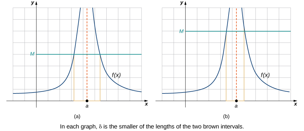
We conclude the process of converting our intuitive ideas of various types of limits to rigorous formal definitions by pursuing a formal definition of infinite limits. To have [latex]\underset{x\to a}{\lim}f(x)=+\infty[/latex], we want the values of the function [latex]f(x)[/latex] to get larger and larger as [latex]x[/latex] approaches [latex]a[/latex]. Instead of the requirement that [latex]|f(x)-L|<\varepsilon[/latex] for arbitrarily small [latex]\varepsilon[/latex] when [latex]0<|x-a|<\delta[/latex] for small enough [latex]\delta[/latex], we want [latex]f(x)>M[/latex] for arbitrarily large positive [latex]M[/latex] when [latex]0<|x-a|<\delta[/latex] for small enough [latex]\delta[/latex]. Figure 6 illustrates this idea by showing the value of [latex]\delta[/latex] for successively larger values of [latex]M[/latex].

Figure 6. These graphs plot values of [latex]\delta[/latex] for [latex]M[/latex] to show that [latex]\underset{x\to a}{\lim}f(x)=+\infty[/latex].