Learning Outcomes
- Apply rates of change to displacement, velocity, and acceleration of an object moving along a straight line.
- Predict the future population from the present value and the population growth rate.
- Use derivatives to calculate marginal cost and revenue in a business situation.
Motion Along a Line
Another use for the derivative is to analyze motion along a line. We have described velocity as the rate of change of position. If we take the derivative of the velocity, we can find the acceleration, or the rate of change of velocity. It is also important to introduce the idea of speed, which is the magnitude of velocity. Thus, we can state the following mathematical definitions.
Definition
Let [latex]s(t)[/latex] be a function giving the position of an object at time [latex]t[/latex].
The velocity of the object at time [latex]t[/latex] is given by [latex]v(t)=s^{\prime}(t)[/latex].
The speed of the object at time [latex]t[/latex] is given by [latex]|v(t)|[/latex].
The acceleration of the object at [latex]t[/latex] is given by [latex]a(t)=v^{\prime}(t)=s''(t)[/latex].
Many of the problems involving position, velocity and acceleration will require finding zeros of quadratic and higher order polynomial functions. To find these zeros, recall that factoring and setting each factor equal to zero will be the easiest way to solve these functions. If it doesn’t factor and it is a quadratic, the quadratic equation will always work.
Example: Comparing Instantaneous Velocity and Average Velocity
A ball is dropped from a height of 64 feet. Its height above ground (in feet) [latex]t[/latex] seconds later is given by [latex]s(t)=-16t^2+64[/latex].
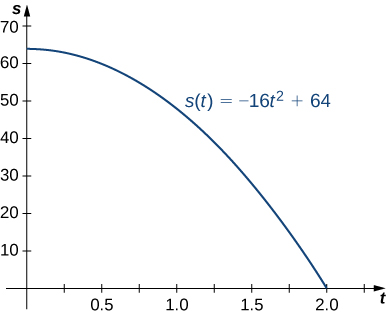
Figure 2. Dropped ball graph, height vs. time.
- What is the instantaneous velocity of the ball when it hits the ground?
- What is the average velocity during its fall?
Example: Interpreting the Relationship between [latex]v(t)[/latex] and [latex]a(t)[/latex]
A particle moves along a coordinate axis in the positive direction to the right. Its position at time [latex]t[/latex] is given by [latex]s(t)=t^3-4t+2[/latex]. Find [latex]v(1)[/latex] and [latex]a(1)[/latex] and use these values to answer the following questions.
- Is the particle moving from left to right or from right to left at time [latex]t=1[/latex]?
- Is the particle speeding up or slowing down at time [latex]t=1[/latex]?
Example: Position and Velocity
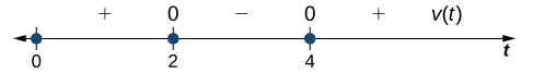
The position of a particle moving along a coordinate axis is given by [latex]s(t)=t^3-9t^2+24t+4, \, t\ge 0[/latex].
- Find [latex]v(t)[/latex].
- At what time(s) is the particle at rest?
- On what time intervals is the particle moving from left to right? From right to left?
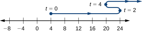
- Use the information obtained to sketch the path of the particle along a coordinate axis.
Watch the following video to see the worked solution to Example: Position and Velocity.
Try It
A particle moves along a coordinate axis. Its position at time [latex]t[/latex] is given by [latex]s(t)=t^2-5t+1[/latex]. Is the particle moving from right to left or from left to right at time [latex]t=3[/latex]?
Try It
Population Change
In addition to analyzing velocity, speed, acceleration, and position, we can use derivatives to analyze various types of populations, including those as diverse as bacteria colonies and cities. We can use a current population, together with a growth rate, to estimate the size of a population in the future. The population growth rate is the rate of change of a population and consequently can be represented by the derivative of the size of the population.
Definition
If [latex]P(t)[/latex] is the number of entities present in a population, then the population growth rate of [latex]P(t)[/latex] is defined to be [latex]P^{\prime}(t)[/latex].
Example: Estimating a Population
The population of a city is tripling every 5 years. If its current population is 10,000, what will be its approximate population 2 years from now?
Watch the following video to see the worked solution to Example: Estimating a Population.
Try It
The current population of a mosquito colony is known to be 3,000; that is, [latex]P(0)=3,000[/latex]. If [latex]P^{\prime}(0)=100[/latex], estimate the size of the population in 3 days, where [latex]t[/latex] is measured in days.
Changes in Cost and Revenue
In addition to analyzing motion along a line and population growth, derivatives are useful in analyzing changes in cost, revenue, and profit. The concept of a marginal function is common in the fields of business and economics and implies the use of derivatives. The marginal cost is the derivative of the cost function. The marginal revenue is the derivative of the revenue function. The marginal profit is the derivative of the profit function, which is based on the cost function and the revenue function.
Definition
If [latex]C(x)[/latex] is the cost of producing [latex]x[/latex] items, then the marginal cost [latex]MC(x)[/latex] is [latex]MC(x)=C^{\prime}(x)[/latex].
If [latex]R(x)[/latex] is the revenue obtained from selling [latex]x[/latex] items, then the marginal revenue [latex]MR(x)[/latex] is [latex]MR(x)=R^{\prime}(x)[/latex].
If [latex]P(x)=R(x)-C(x)[/latex] is the profit obtained from selling [latex]x[/latex] items, then the marginal profit [latex]MP(x)[/latex] is defined to be [latex]MP(x)=P^{\prime}(x)=MR(x)-MC(x)=R^{\prime}(x)-C^{\prime}(x)[/latex].
We can roughly approximate
by choosing an appropriate value for [latex]h[/latex]. Since [latex]x[/latex] represents objects, a reasonable and small value for [latex]h[/latex] is 1. Thus, by substituting [latex]h=1[/latex], we get the approximation [latex]MC(x)=C^{\prime}(x)\approx C(x+1)-C(x)[/latex]. Consequently, [latex]C^{\prime}(x)[/latex] for a given value of [latex]x[/latex] can be thought of as the change in cost associated with producing one additional item. In a similar way, [latex]MR(x)=R^{\prime}(x)[/latex] approximates the revenue obtained by selling one additional item, and [latex]MP(x)=P^{\prime}(x)[/latex] approximates the profit obtained by producing and selling one additional item.
Example: Applying Marginal Revenue
Assume that the number of barbeque dinners that can be sold, [latex]x[/latex], can be related to the price charged, [latex]p[/latex], by the equation [latex]p(x)=9-0.03x, \, 0\le x\le 300[/latex].
In this case, the revenue in dollars obtained by selling [latex]x[/latex] barbeque dinners is given by
Use the marginal revenue function to estimate the revenue obtained from selling the 101st barbeque dinner. Compare this to the actual revenue obtained from the sale of this dinner.
Watch the following video to see the worked solution to Example: Applying Marginal Revenue.
Try It
Suppose that the profit obtained from the sale of [latex]x[/latex] fish-fry dinners is given by [latex]P(x)=-0.03x^2+8x-50[/latex]. Use the marginal profit function to estimate the profit from the sale of the 101st fish-fry dinner.
Candela Citations
- 3.4 Derivatives as Rates of Change. Authored by: Ryan Melton. License: CC BY: Attribution
- Calculus Volume 1. Authored by: Gilbert Strang, Edwin (Jed) Herman. Provided by: OpenStax. Located at: https://openstax.org/details/books/calculus-volume-1. License: CC BY-NC-SA: Attribution-NonCommercial-ShareAlike. License Terms: Access for free at https://openstax.org/books/calculus-volume-1/pages/1-introduction
