Learning Outcomes
- Explain how the sign of the first derivative affects the shape of a function’s graph
- State the first derivative test for critical points
- Use concavity and inflection points to explain how the sign of the second derivative affects the shape of a function’s graph
- Explain the concavity test for a function over an open interval
The First Derivative Test
Corollary 3 of the Mean Value Theorem showed that if the derivative of a function is positive over an interval [latex]I[/latex] then the function is increasing over [latex]I[/latex]. On the other hand, if the derivative of the function is negative over an interval [latex]I[/latex], then the function is decreasing over [latex]I[/latex] as shown in the following figure.
Figure 1. Both functions are increasing over the interval [latex](a,b)[/latex]. At each point [latex]x[/latex], the derivative [latex]f^{\prime}(x)>0[/latex]. Both functions are decreasing over the interval [latex](a,b)[/latex]. At each point [latex]x[/latex], the derivative [latex]f^{\prime}(x)<0[/latex].
A continuous function [latex]f[/latex] has a local maximum at point [latex]c[/latex] if and only if [latex]f[/latex] switches from increasing to decreasing at point [latex]c[/latex]. Similarly, [latex]f[/latex] has a local minimum at [latex]c[/latex] if and only if [latex]f[/latex] switches from decreasing to increasing at [latex]c[/latex]. If [latex]f[/latex] is a continuous function over an interval [latex]I[/latex] containing [latex]c[/latex] and differentiable over [latex]I[/latex], except possibly at [latex]c[/latex], the only way [latex]f[/latex] can switch from increasing to decreasing (or vice versa) at point [latex]c[/latex] is if [latex]{f}^{\prime }[/latex] changes sign as [latex]x[/latex] increases through [latex]c.[/latex] If [latex]f[/latex] is differentiable at [latex]c,[/latex] the only way that [latex]{f}^{\prime }.[/latex] can change sign as [latex]x[/latex] increases through [latex]c[/latex] is if [latex]f^{\prime}(c)=0[/latex]. Therefore, for a function [latex]f[/latex] that is continuous over an interval [latex]I[/latex] containing [latex]c[/latex] and differentiable over [latex]I[/latex], except possibly at [latex]c[/latex], the only way [latex]f[/latex] can switch from increasing to decreasing (or vice versa) is if [latex]f^{\prime}(c)=0[/latex] or [latex]f^{\prime}(c)[/latex] is undefined. Consequently, to locate local extrema for a function [latex]f[/latex], we look for points [latex]c[/latex] in the domain of [latex]f[/latex] such that [latex]f^{\prime}(c)=0[/latex] or [latex]f^{\prime}(c)[/latex] is undefined. Recall that such points are called critical points of [latex]f[/latex].
Note that [latex]f[/latex] need not have a local extrema at a critical point. The critical points are candidates for local extrema only. In Figure 2, we show that if a continuous function [latex]f[/latex] has a local extremum, it must occur at a critical point, but a function may not have a local extremum at a critical point. We show that if [latex]f[/latex] has a local extremum at a critical point, then the sign of [latex]f^{\prime}[/latex] switches as [latex]x[/latex] increases through that point.
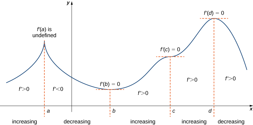
Figure 2. The function [latex]f[/latex] has four critical points: [latex]a,b,c[/latex], and [latex]d[/latex]. The function [latex]f[/latex] has local maxima at [latex]a[/latex] and [latex]d[/latex], and a local minimum at [latex]b[/latex]. The function [latex]f[/latex] does not have a local extremum at [latex]c[/latex]. The sign of [latex]f^{\prime}[/latex] changes at all local extrema.
Using Figure 2, we summarize the main results regarding local extrema.
- If a continuous function [latex]f[/latex] has a local extremum, it must occur at a critical point [latex]c[/latex].
- The function has a local extremum at the critical point [latex]c[/latex] if and only if the derivative [latex]f^{\prime}[/latex] switches sign as [latex]x[/latex] increases through [latex]c[/latex].
- Therefore, to test whether a function has a local extremum at a critical point [latex]c[/latex], we must determine the sign of [latex]f^{\prime}(x)[/latex] to the left and right of [latex]c[/latex].
This result is known as the first derivative test.
First Derivative Test
Suppose that [latex]f[/latex] is a continuous function over an interval [latex]I[/latex] containing a critical point [latex]c[/latex]. If [latex]f[/latex] is differentiable over [latex]I[/latex], except possibly at point [latex]c[/latex], then [latex]f(c)[/latex] satisfies one of the following descriptions:
- If [latex]f^{\prime}[/latex] changes sign from positive when [latex]x
- If [latex]f^{\prime}[/latex] changes sign from negative when [latex]x
- If [latex]f^{\prime}[/latex] has the same sign for [latex]x
We can summarize the first derivative test as a strategy for locating local extrema.
Problem-Solving Strategy: Using the First Derivative Test
Consider a function [latex]f[/latex] that is continuous over an interval [latex]I[/latex].
- Find all critical points of [latex]f[/latex] and divide the interval [latex]I[/latex] into smaller intervals using the critical points as endpoints.
- Analyze the sign of [latex]f^{\prime}[/latex] in each of the subintervals. If [latex]f^{\prime}[/latex] is continuous over a given subinterval (which is typically the case), then the sign of [latex]f^{\prime}[/latex] in that subinterval does not change and, therefore, can be determined by choosing an arbitrary test point [latex]x[/latex] in that subinterval and by evaluating the sign of [latex]f^{\prime}[/latex] at that test point. Use the sign analysis to determine whether [latex]f[/latex] is increasing or decreasing over that interval.
- Use the first derivative test and the results of step 2 to determine whether [latex]f[/latex] has a local maximum, a local minimum, or neither at each of the critical points.
Recall from Chapter 4.3 that when talking about local extrema, the value of the extremum is the y value and the location of the extremum is the x value.
Now let’s look at how to use this strategy to locate all local extrema for particular functions.
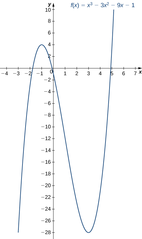
Example: Using the First Derivative Test to Find Local Extrema
Use the first derivative test to find the location of all local extrema for [latex]f(x)=x^3-3x^2-9x-1[/latex]. Use a graphing utility to confirm your results.
Watch the following video to see the worked solution to Example: Using the First Derivative Test to Find Local Extrema.
Try It
Use the first derivative test to locate all local extrema for [latex]f(x)=−x^3+\frac{3}{2}x^2+18x[/latex].
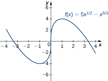
Example: Using the First Derivative Test
Use the first derivative test to find the location of all local extrema for [latex]f(x)=5x^{\frac{1}{3}}-x^{\frac{5}{3}}[/latex]. Use a graphing utility to confirm your results.
Try It
Use the first derivative test to find all local extrema for [latex]f(x)=\sqrt[3]{x-1}[/latex].
Try It
Try It
Concavity and Points of Inflection
We now know how to determine where a function is increasing or decreasing. However, there is another issue to consider regarding the shape of the graph of a function. If the graph curves, does it curve upward or curve downward? This notion is called the concavity of the function.
Figure 5(a) shows a function [latex]f[/latex] with a graph that curves upward. As [latex]x[/latex] increases, the slope of the tangent line increases. Thus, since the derivative increases as [latex]x[/latex] increases, [latex]f^{\prime}[/latex] is an increasing function. We say this function [latex]f[/latex] is concave up. Figure 5(b) shows a function [latex]f[/latex] that curves downward. As [latex]x[/latex] increases, the slope of the tangent line decreases. Since the derivative decreases as [latex]x[/latex] increases, [latex]f^{\prime}[/latex] is a decreasing function. We say this function [latex]f[/latex] is concave down.
Definition
Let [latex]f[/latex] be a function that is differentiable over an open interval [latex]I[/latex]. If [latex]f^{\prime}[/latex] is increasing over [latex]I[/latex], we say [latex]f[/latex] is concave up over [latex]I[/latex]. If [latex]f^{\prime}[/latex] is decreasing over [latex]I[/latex], we say [latex]f[/latex] is concave down over [latex]I[/latex].
Figure 5. (a), (c) Since [latex]f^{\prime}[/latex] is increasing over the interval [latex](a,b)[/latex], we say [latex]f[/latex] is concave up over [latex](a,b)[/latex]. (b), (d) Since [latex]f^{\prime}[/latex] is decreasing over the interval [latex](a,b)[/latex], we say [latex]f[/latex] is concave down over [latex](a,b)[/latex].
In general, without having the graph of a function [latex]f[/latex], how can we determine its concavity? By definition, a function [latex]f[/latex] is concave up if [latex]f^{\prime}[/latex] is increasing. From Corollary 3, we know that if [latex]f^{\prime}[/latex] is a differentiable function, then [latex]f^{\prime}[/latex] is increasing if its derivative [latex]f^{\prime \prime}(x)>0[/latex]. Therefore, a function [latex]f[/latex] that is twice differentiable is concave up when [latex]f^{\prime \prime}(x)>0[/latex]. Similarly, a function [latex]f[/latex] is concave down if [latex]f^{\prime}[/latex] is decreasing. We know that a differentiable function [latex]f^{\prime}[/latex] is decreasing if its derivative [latex]f^{\prime \prime}(x)<0[/latex]. Therefore, a twice-differentiable function [latex]f[/latex] is concave down when [latex]f^{\prime \prime}(x)<0[/latex]. Applying this logic is known as the concavity test.
Test for Concavity
Let [latex]f[/latex] be a function that is twice differentiable over an interval [latex]I[/latex].
- If [latex]f^{\prime \prime}(x)>0[/latex] for all [latex]x \in I[/latex], then [latex]f[/latex] is concave up over [latex]I[/latex].
- If [latex]f^{\prime \prime}(x)<0[/latex] for all [latex]x \in I[/latex], then [latex]f[/latex] is concave down over [latex]I[/latex].
We conclude that we can determine the concavity of a function [latex]f[/latex] by looking at the second derivative of [latex]f[/latex]. In addition, we observe that a function [latex]f[/latex] can switch concavity (Figure 6). However, a continuous function can switch concavity only at a point [latex]x[/latex] if [latex]f^{\prime \prime}(x)=0[/latex] or [latex]f^{\prime \prime}(x)[/latex] is undefined. Consequently, to determine the intervals where a function [latex]f[/latex] is concave up and concave down, we look for those values of [latex]x[/latex] where [latex]f^{\prime \prime}(x)=0[/latex] or [latex]f^{\prime \prime}(x)[/latex] is undefined. When we have determined these points, we divide the domain of [latex]f[/latex] into smaller intervals and determine the sign of [latex]f^{\prime \prime}[/latex] over each of these smaller intervals. If [latex]f^{\prime \prime}[/latex] changes sign as we pass through a point [latex]x[/latex], then [latex]f[/latex] changes concavity. It is important to remember that a function [latex]f[/latex] may not change concavity at a point [latex]x[/latex] even if [latex]f^{\prime \prime}(x)=0[/latex] or [latex]f^{\prime \prime}(x)[/latex] is undefined. If, however, [latex]f[/latex] does change concavity at a point [latex]a[/latex] and [latex]f[/latex] is continuous at [latex]a[/latex], we say the point [latex](a,f(a))[/latex] is an inflection point of [latex]f[/latex].
Definition
If [latex]f[/latex] is continuous at [latex]a[/latex] and [latex]f[/latex] changes concavity at [latex]a[/latex], the point [latex](a,f(a))[/latex] is an inflection point of [latex]f[/latex].
Figure 6. Since [latex]f^{\prime \prime}(x)>0[/latex] for [latex]x<a[/latex], the function [latex]f[/latex] is concave up over the interval [latex](−\infty,a)[/latex]. Since [latex]f^{\prime \prime}(x)<0[/latex] for [latex]x>a[/latex], the function [latex]f[/latex] is concave down over the interval [latex](a,\infty)[/latex]. The point [latex](a,f(a))[/latex] is an inflection point of [latex]f[/latex].
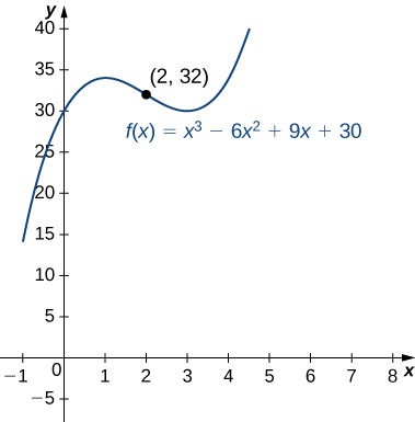
Example: Testing for Concavity
For the function [latex]f(x)=x^3-6x^2+9x+30[/latex], determine all intervals where [latex]f[/latex] is concave up and all intervals where [latex]f[/latex] is concave down. List all inflection points for [latex]f[/latex]. Use a graphing utility to confirm your results.
Watch the following video to see the worked solution to Example: Testing for Concavity.
Try It
For [latex]f(x)=−x^3+\frac{3}{2}x^2+18x[/latex], find all intervals where [latex]f[/latex] is concave up and all intervals where [latex]f[/latex] is concave down.
We now summarize, in the box below, the information that the first and second derivatives of a function [latex]f[/latex] provide about the graph of [latex]f[/latex], and illustrate this information in Figure 8.
| Sign of [latex]f^{\prime}[/latex] | Sign of [latex]f^{\prime \prime}[/latex] | Is [latex]f[/latex] increasing or decreasing? | Concavity |
|---|---|---|---|
| Positive | Positive | Increasing | Concave up |
| Positive | Negative | Increasing | Concave down |
| Negative | Positive | Decreasing | Concave up |
| Negative | Negative | Decreasing | Concave down |
Figure 8. Consider a twice-differentiable function [latex]f[/latex] over an open interval [latex]I[/latex]. If [latex]f^{\prime}(x)>0[/latex] for all [latex]x \in I[/latex], the function is increasing over [latex]I[/latex]. If [latex]f^{\prime}(x)<0[/latex] for all [latex]x \in I[/latex], the function is decreasing over [latex]I[/latex]. If [latex]f^{\prime \prime}(x)>0[/latex] for all [latex]x \in I[/latex], the function is concave up. If [latex]f^{\prime \prime}(x)<0[/latex] for all [latex]x \in I[/latex], the function is concave down on [latex]I[/latex].
Candela Citations
- 4.5 Derivatives and the Shape of a Graph. Authored by: Ryan Melton. License: CC BY: Attribution
- Calculus Volume 1. Authored by: Gilbert Strang, Edwin (Jed) Herman. Provided by: OpenStax. Located at: https://openstax.org/details/books/calculus-volume-1. License: CC BY-NC-SA: Attribution-NonCommercial-ShareAlike. License Terms: Access for free at https://openstax.org/books/calculus-volume-1/pages/1-introduction
