The Squeeze Theorem

Learning Outcomes

Evaluate the limit of a function by using the squeeze theorem

The techniques we have developed thus far work very well for algebraic functions, but we are still unable to evaluate limits of very basic trigonometric functions. The next theorem, called the squeeze theorem, proves very useful for establishing basic trigonometric limits. This theorem allows us to calculate limits by “squeezing” a function, with a limit at a point $a$ that is unknown, between two functions having a common known limit at $a$ . Figure 5 illustrates this idea.

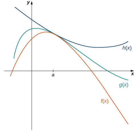
A graph of three functions over a small interval. All three functions curve. Over this interval, the function g(x) is trapped between the functions h(x), which gives greater y values for the same x values, and f(x), which gives smaller y values for the same x values. The functions all approach the same limit when x=a.

Figure 5. The Squeeze Theorem applies when $f(x)\le g(x)\le h(x)$ and $\underset{x\to a}{\lim}f(x)=\underset{x\to a}{\lim}h(x)$ .

Let $f(x), \, g(x)$ , and $h(x)$ be defined for all $x\ne a$ over an open interval containing $a$ . If

f (x) \leq g (x) \leq h (x)

$f(x)\le g(x)\le h(x)$

for all $x\ne a$ in an open interval containing $a$ and

lim_{x \to a} f (x) = L = lim_{x \to a} h (x)

$\underset{x\to a}{\lim}f(x)=L=\underset{x\to a}{\lim}h(x)$

where $L$ is a real number, then $\underset{x\to a}{\lim}g(x)=L$ .

Example: Applying the Squeeze Theorem

Apply the Squeeze Theorem to evaluate $\underset{x\to 0}{\lim}x \cos x$ .

Show Solution

Because $-1\le \cos x\le 1$ for all $x$ , we have $-|x|\le x \cos x\le |x|$ . Since $\underset{x\to 0}{\lim}(-|x|)=0=\underset{x\to 0}{\lim}|x|$ , from the Squeeze Theorem, we obtain $\underset{x\to 0}{\lim}x \cos x=0$ . The graphs of $f(x)=-|x|, \, g(x)=x \cos x$ , and $h(x)=|x|$ are shown in Figure 6.

The graph of three functions: h(x) = x, f(x) = -x, and g(x) = xcos(x). The first, h(x) = x, is a linear function with slope of 1 going through the origin. The second, f(x), is also a linear function with slope of −1; going through the origin. The third, g(x) = xcos(x), curves between the two and goes through the origin. It opens upward for x>0 and downward for x>0.

Figure 6. The graphs of 𝑓(𝑥), 𝑔(𝑥), and ℎ(𝑥) are shown around the point 𝑥=0.

Try It

Use the Squeeze Theorem to evaluate $\underset{x\to 0}{\lim}x^2 \sin \dfrac{1}{x}$ .

Hint

Use the fact that $-x^2\le x^2 \sin (\frac{1}{x})\le x^2$ to help you find two functions such that $x^2 \sin (\frac{1}{x})$ is squeezed between them.

Show Solution

Watch the following video to see the worked solution to the above Try It.

Closed Captioning and Transcript Information for Video

We now use the squeeze theorem to tackle several very important limits. Although this discussion is somewhat lengthy, these limits prove invaluable for the development of the material in both the next section and the next module. The first of these limits is $\underset{\theta \to 0}{\lim} \sin \theta$ . Consider the unit circle shown in Figure 7. In the figure, we see that $\sin \theta$ is the $y$ -coordinate on the unit circle and it corresponds to the line segment shown in blue. The radian measure of angle θ is the length of the arc it subtends on the unit circle. Therefore, we see that for $0<\theta <\frac{\pi }{2}, \, 0 < \sin \theta < \theta$ .

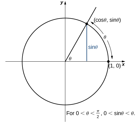
A diagram of the unit circle in the x,y plane – it is a circle with radius 1 and center at the origin. A specific point (cos(theta), sin(theta)) is labeled in quadrant 1 on the edge of the circle. This point is one vertex of a right triangle inside the circle, with other vertices at the origin and (cos(theta), 0). As such, the lengths of the sides are cos(theta) for the base and sin(theta) for the height, where theta is the angle created by the hypotenuse and base. The radian measure of angle theta is the length of the arc it subtends on the unit circle. The diagram shows that for 0 < theta < pi/2, 0 < sin(theta) < theta.

Figure 7. The sine function is shown as a line on the unit circle.

Because $\underset{\theta \to 0^+}{\lim}0=0$ and $\underset{\theta \to 0^+}{\lim}\theta =0$ , by using the Squeeze Theorem we conclude that

lim_{θ \to 0^{+}} \sin θ = 0

$\underset{\theta \to 0^+}{\lim} \sin \theta =0$

To see that $\underset{\theta \to 0^-}{\lim} \sin \theta =0$ as well, observe that for $-\frac{\pi }{2} < \theta <0, \, 0 < −\theta < \frac{\pi}{2}$ and hence, $0 < \sin(-\theta) < −\theta$ . Consequently, $0 < -\sin \theta < −\theta$ It follows that $0 > \sin \theta > \theta$ . An application of the Squeeze Theorem produces the desired limit. Thus, since $\underset{\theta \to 0^+}{\lim} \sin \theta =0$ and $\underset{\theta \to 0^-}{\lim} \sin \theta =0$ ,

lim_{θ \to 0} \sin θ = 0

$\underset{\theta \to 0}{\lim} \sin \theta =0$

Next, using the identity $\cos \theta =\sqrt{1-\sin^2 \theta}$ for $-\frac{\pi}{2}<\theta <\frac{\pi}{2}$ , we see that

lim_{θ \to 0} \cos θ = lim_{θ \to 0} \sqrt{1 - \sin^{2} θ} = 1

$\underset{\theta \to 0}{\lim} \cos \theta =\underset{\theta \to 0}{\lim}\sqrt{1-\sin^2 \theta }=1$

We now take a look at a limit that plays an important role in later modules—namely, $\underset{\theta \to 0}{\lim}\frac{\sin \theta}{\theta}$ . To evaluate this limit, we use the unit circle in Figure 7. Notice that this figure adds one additional triangle to Figure 8. We see that the length of the side opposite angle $\theta$ in this new triangle is $\tan \theta$ . Thus, we see that for $0 < \theta < \frac{\pi}{2}, \, \sin \theta < \theta < \tan \theta$ .

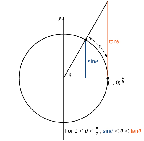
The same diagram as the previous one. However, the triangle is expanded. The base is now from the origin to (1,0). The height goes from (1,0) to (1, tan(theta)). The hypotenuse goes from the origin to (1, tan(theta)). As such, the height is now tan(theta). It shows that for 0 < theta < pi/2, sin(theta) < theta < tan(theta).

Figure 8. The sine and tangent functions are shown as lines on the unit circle.

By dividing by $\sin \theta$ in all parts of the inequality, we obtain

1 < \frac{θ}{\sin θ} < \frac{1}{\cos θ}

$1 < \dfrac{\theta}{\sin \theta} < \dfrac{1}{\cos \theta}$

Equivalently, we have

1 > \frac{\sin θ}{θ} > \cos θ

$1 > \dfrac{\sin \theta}{\theta} > \cos \theta$

Since $\underset{\theta \to 0^+}{\lim}1=1=\underset{\theta \to 0^+}{\lim}\cos \theta$ , we conclude that $\underset{\theta \to 0^+}{\lim}\frac{\sin \theta}{\theta}=1$ . By applying a manipulation similar to that used in demonstrating that $\underset{\theta \to 0^-}{\lim}\sin \theta =0$ , we can show that $\underset{\theta \to 0^-}{\lim}\frac{\sin \theta}{\theta}=1$ . Thus,

lim_{θ \to 0} \frac{\sin θ}{θ} = 1

$\underset{\theta \to 0}{\lim}\dfrac{\sin \theta}{\theta}=1$

In the example below, we use this limit to establish $\underset{\theta \to 0}{\lim}\frac{1- \cos \theta}{\theta}=0$ . This limit also proves useful in later modules.

Example: Evaluating an Important Trigonometric Limit

Evaluate $\underset{\theta \to 0}{\lim}\dfrac{1- \cos \theta}{\theta}$

Show Solution

In the first step, we multiply by the conjugate so that we can use a trigonometric identity to convert the cosine in the numerator to a sine:

\begin{array}{cc} lim_{θ \to 0} \frac{1 - \cos θ}{θ} & = lim_{θ \to 0} \frac{1 - \cos θ}{θ} \cdot \frac{1 + \cos θ}{1 + \cos θ} \\ = lim_{θ \to 0} \frac{1 - \cos^{2} θ}{θ (1 + \cos θ)} \\ = lim_{θ \to 0} \frac{\sin^{2} θ}{θ (1 + \cos θ)} \\ = lim_{θ \to 0} \frac{\sin θ}{θ} \cdot \frac{\sin θ}{1 + \cos θ} \\ = 1 \cdot \frac{0}{2} = 0 \end{array}

$\begin{array}{cc} \underset{\theta \to 0}{\lim}\frac{1- \cos \theta}{\theta}& =\underset{\theta \to 0}{\lim}\frac{1- \cos \theta}{\theta} \cdot \frac{1+ \cos \theta}{1+ \cos \theta} \\ & =\underset{\theta \to 0}{\lim}\frac{1-\cos^2 \theta}{\theta(1+ \cos \theta)} \\ & =\underset{\theta \to 0}{\lim}\frac{\sin^2 \theta}{\theta(1+ \cos \theta)} \\ & =\underset{\theta \to 0}{\lim}\frac{\sin \theta}{\theta} \cdot \frac{\sin \theta}{1+ \cos \theta} \\ & =1 \cdot \frac{0}{2}=0 \end{array}$

Therefore,

lim_{θ \to 0} \frac{1 - \cos θ}{θ} = 0

$\underset{\theta \to 0}{\lim}\dfrac{1- \cos \theta}{\theta}=0$

Watch the following video to see the worked solution to Example: Evaluating an Important Trigonometric Limit

Closed Captioning and Transcript Information for Video

Try It

Evaluate $\underset{\theta \to 0}{\lim}\dfrac{1- \cos \theta}{\sin \theta}$

Hint

Multiply numerator and denominator by $1+ \cos \theta$ .

Show Solution

Try It

Activity: Deriving the Formula for the Area of a Circle

Some of the geometric formulas we take for granted today were first derived by methods that anticipate some of the methods of calculus. The Greek mathematician Archimedes (ca. 287−212 BCE) was particularly inventive, using polygons inscribed within circles to approximate the area of the circle as the number of sides of the polygon increased. He never came up with the idea of a limit, but we can use this idea to see what his geometric constructions could have predicted about the limit.

We can estimate the area of a circle by computing the area of an inscribed regular polygon. Think of the regular polygon as being made up of $n$ triangles. By taking the limit as the vertex angle of these triangles goes to zero, you can obtain the area of the circle. To see this, carry out the following steps:

Express the height $h$ and the base $b$ of the isosceles triangle in Figure 9 in terms of $\theta$ and $r$ .

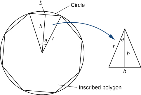
Figure 9.
Using the expressions that you obtained in step 1, express the area of the isosceles triangle in terms of $\theta$ and $r$ .
(Substitute $(\frac{1}{2})\sin \theta$ for $\sin(\frac{\theta}{2}) \cos(\frac{\theta}{2})$ in your expression.)
If an $n$ -sided regular polygon is inscribed in a circle of radius $r$ , find a relationship between $\theta$ and $n$ . Solve this for $n$ . Keep in mind there are $2\pi$ radians in a circle. (Use radians, not degrees.)
Find an expression for the area of the $n$ -sided polygon in terms of $r$ and $\theta$ .
To find a formula for the area of the circle, find the limit of the expression in step 4 as $\theta$ goes to zero. (Hint: $\underset{\theta \to 0}{\lim}\frac{(\sin \theta)}{\theta}=1$ .)

The technique of estimating areas of regions by using polygons is revisited in Module 5: Integration.

Module 2: Limits