Learning Objectives
- Use Stokes’ theorem to evaluate a line integral.
- Use Stokes’ theorem to calculate a surface integral.
- Use Stokes’ theorem to calculate a curl.
Applying Stokes’ Theorem
Stokes’ theorem translates between the flux integral of surface [latex]S[/latex] to a line integral around the boundary of [latex]S[/latex]. Therefore, the theorem allows us to compute surface integrals or line integrals that would ordinarily be quite difficult by translating the line integral into a surface integral or vice versa. We now study some examples of each kind of translation.
Example: calculating a surface integral
Calculate surface integral [latex]\displaystyle\iint_S\text{curl }{\bf{F}}\cdot{d}{\bf{S}}[/latex], where [latex]S[/latex] is the surface, oriented outward, in Figure 1 and [latex]{\bf{F}}=\langle{z},2xy,x+y\rangle[/latex].
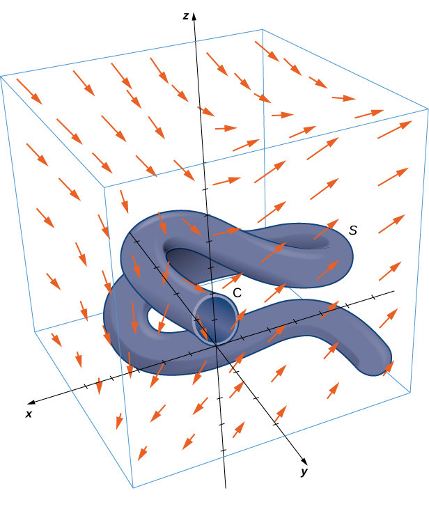
Figure 1. A complicated surface in a vector field.
An amazing consequence of Stokes’ theorem is that if [latex]S'[/latex] is any other smooth surface with boundary [latex]C[/latex] and the same orientation as [latex]S[/latex], then [latex]\displaystyle\iint_S\text{curl }{\bf{F}}\cdot{d}{\bf{S}}=\displaystyle\int_C{\bf{F}}\cdot{d}{\bf{r}}=0[/latex] because Stokes’ theorem says the surface integral depends on the line integral around the boundary only.
In Example “Calculating a Surface Integral”, we calculated a surface integral simply by using information about the boundary of the surface. In general, let [latex]S_1[/latex] and [latex]S_2[/latex] be smooth surfaces with the same boundary [latex]C[/latex] and the same orientation. By Stokes’ theorem,
[latex]\large{\displaystyle\iint_{S_1}\text{curl }{\bf{F}}\cdot{d}{\bf{S}}=\displaystyle\int_C{\bf{F}}\cdot{d}{\bf{r}}=\displaystyle\iint_{S_2}\text{curl }{\bf{F}}\cdot{d}{\bf{S}}}[/latex].
Therefore, if [latex]\displaystyle\iint_{S_1}\text{curl }{\bf{F}}\cdot{d}{\bf{S}}[/latex] is difficult to calculate but [latex]\displaystyle\iint_{S_2}\text{curl }{\bf{F}}\cdot{d}{\bf{S}}[/latex] is easy to calculate, Stokes’ theorem allows us to calculate the easier surface integral. In Example “Calculating a Surface Integral”, we could have calculated [latex]\displaystyle\iint_{S}\text{curl }{\bf{F}}\cdot{d}{\bf{S}}[/latex] by calculating [latex]\displaystyle\iint_{S^\prime}\text{curl }{\bf{F}}\cdot{d}{\bf{S}}[/latex], where [latex]S'[/latex] is the disk enclosed by boundary curve [latex]C[/latex] (a much more simple surface with which to work).
[latex]{\displaystyle\iint_{S_1}\text{curl }{\bf{F}}\cdot{d}{\bf{S}}=\displaystyle\int_C{\bf{F}}\cdot{d}{\bf{r}}=\displaystyle\iint_{S_2}\text{curl }{\bf{F}}\cdot{d}{\bf{S}}}[/latex] shows that flux integrals of curl vector fields are surface independent in the same way that line integrals of gradient fields are path independent. Recall that if [latex]{\bf{F}}[/latex] is a two-dimensional conservative vector field defined on a simply connected domain, [latex]f[/latex] is a potential function for [latex]{\bf{F}}[/latex], and [latex]C[/latex] is a curve in the domain of [latex]{\bf{F}}[/latex], then [latex]\displaystyle\int_C{\bf{F}}\cdot{d}{\bf{r}}[/latex] depends only on the endpoints of [latex]C[/latex]. Therefore if [latex]C'[/latex] is any other curve with the same starting point and endpoint as [latex]C[/latex] (that is, [latex]C'[/latex] has the same orientation as [latex]C[/latex]), then [latex]\displaystyle\int_C{\bf{F}}\cdot{d}{\bf{r}}=\displaystyle\int_{C^\prime}{\bf{F}}\cdot{d}{\bf{r}}[/latex]. In other words, the value of the integral depends on the boundary of the path only; it does not really depend on the path itself.
Analogously, suppose that [latex]S[/latex] and [latex]S'[/latex] are surfaces with the same boundary and same orientation, and suppose that [latex]{\bf{G}}[/latex] is a three-dimensional vector field that can be written as the curl of another vector field [latex]{\bf{F}}[/latex] (so that [latex]{\bf{F}}[/latex] is like a “potential field” of [latex]{\bf{G}}[/latex]). By [latex]{\displaystyle\iint_{S_1}\text{curl }{\bf{F}}\cdot{d}{\bf{S}}=\displaystyle\int_C{\bf{F}}\cdot{d}{\bf{r}}=\displaystyle\iint_{S_2}\text{curl }{\bf{F}}\cdot{d}{\bf{S}}}[/latex],
[latex]\large{\displaystyle\int_S{\bf{G}}\cdot{d}{\bf{S}}=\displaystyle\iint_{S}\text{curl }{\bf{F}}\cdot{d}{\bf{S}}=\displaystyle\int_C{\bf{F}}\cdot{d}{\bf{r}}=\displaystyle\iint_{S^\prime}\text{curl }{\bf{F}}\cdot{d}{\bf{S}}=\displaystyle\iint_{S^\prime}\text{curl }{\bf{G}}\cdot{d}{\bf{S}}}[/latex].
Therefore, the flux integral of [latex]{\bf{G}}[/latex] does not depend on the surface, only on the boundary of the surface. Flux integrals of vector fields that can be written as the curl of a vector field are surface independent in the same way that line integrals of vector fields that can be written as the gradient of a scalar function are path independent.
try it
Use Stokes’ theorem to calculate surface integral [latex]\displaystyle\iint_{S}\text{curl }{\bf{F}}\cdot{d}{\bf{S}}[/latex], where [latex]{\bf{F}}=\langle{z},x,y\rangle[/latex] and [latex]S[/latex] is the surface as shown in the following figure. The boundary curve, [latex]C[/latex], is oriented clockwise when looking along the positive [latex]y[/latex]-axis.

Example: calculating a line integral
Calculate the line integral [latex]\displaystyle\int_C{\bf{F}}\cdot{d}{\bf{r}}[/latex], where [latex]{\bf{F}}=\langle{x}y,x^2+y^2+z^2,yz\rangle[/latex] and [latex]C[/latex] is the boundary of the parallelogram with vertices [latex](0, 0, 1)[/latex], [latex](0, 1, 0)[/latex], [latex](2, 0, -1)[/latex], and [latex](2, 1, -2)[/latex].
try it
Use Stokes’ theorem to calculate line integral [latex]\displaystyle\int_C{\bf{F}}\cdot{d}{\bf{r}}[/latex], where [latex]{\bf{F}}=\langle{z},x,y\rangle[/latex] and [latex]C[/latex] is oriented clockwise and is the boundary of a triangle with vertices [latex](0, 0, 1)[/latex], [latex](3, 0, -2)[/latex], and [latex](0, 1, 2)[/latex].
Watch the following video to see the worked solution to the above Try It
Interpretation of Curl
In addition to translating between line integrals and flux integrals, Stokes’ theorem can be used to justify the physical interpretation of curl that we have learned. Here we investigate the relationship between curl and circulation, and we use Stokes’ theorem to state Faraday’s law—an important law in electricity and magnetism that relates the curl of an electric field to the rate of change of a magnetic field.
Recall that if [latex]C[/latex] is a closed curve and [latex]{\bf{F}}[/latex] is a vector field defined on [latex]C[/latex], then the circulation of [latex]{\bf{F}}[/latex] around [latex]C[/latex] is line integral [latex]\displaystyle\int_C{\bf{F}}\cdot{d}{\bf{r}}[/latex]. If [latex]{\bf{F}}[/latex] represents the velocity field of a fluid in space, then the circulation measures the tendency of the fluid to move in the direction of [latex]C[/latex].
Let [latex]{\bf{F}}[/latex] be a continuous vector field and let [latex]D_r[/latex] be a small disk of radius [latex]r[/latex] with center [latex]P_0[/latex] (Figure 2). If [latex]D_r[/latex] is small enough, then [latex](\text{curl }{\bf{F}})(P)\approx(\text{curl }{\bf{F}})(P_0)[/latex] for all points [latex]P[/latex] in [latex]D_r[/latex] because the curl is continuous. Let [latex]C_r[/latex] be the boundary circle of [latex]D_r[/latex]. By Stokes’ theorem,
[latex]\large{\displaystyle\int_{C_r}{\bf{F}}\cdot{d}{\bf{r}}=\displaystyle\iint_{D_r}\text{curl }{\bf{F}}\cdot{\bf{N}}{d}S\approx\displaystyle\iint_{D_r}(\text{curl }{\bf{F}})(P_0)\cdot{\bf{N}}(P_0)dS}[/latex].
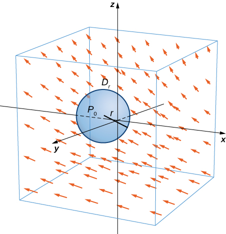
Figure 2. Disk [latex]{D_r}[/latex] is a small disk in a continuous vector field.
The quantity [latex](\text{curl }{\bf{F}})(P_0)\cdot{\bf{N}}(P_0)[/latex] is constant, and therefore
[latex]\large{\displaystyle\iint_{D_r}(\text{curl }{\bf{F}})(P_0)\cdot{\bf{N}}(P_0)dS=\pi{r}^2[(\text{curl }{\bf{F}})(P_0)\cdot{\bf{N}}(P_0)]}[/latex].
Thus
[latex]\large{\displaystyle\int_{C_r}{\bf{F}}\cdot{d}{\bf{r}}\approx\pi{r}^2[(\text{curl }{\bf{F}})(P_0)\cdot{\bf{N}}(P_0)]}[/latex],
and the approximation gets arbitrarily close as the radius shrinks to zero. Therefore Stokes’ theorem implies that
[latex]\large{(\text{curl }{\bf{F}})(P_0)\cdot{\bf{N}}(P_0)=\displaystyle\lim_{r\to0^+}\frac{1}{\pi{r^2}}\displaystyle\int_{C_r}{\bf{F}}\cdot{d}{\bf{r}}}[/latex].
This equation relates the curl of a vector field to the circulation. Since the area of the disk is [latex]\pi{r}^2[/latex], this equation says we can view the curl (in the limit) as the circulation per unit area. Recall that if [latex]{\bf{F}}[/latex] is the velocity field of a fluid, then circulation [latex]\displaystyle\oint_{c_r}{\bf{F}}\cdot{d}{\bf{r}}=\displaystyle\oint_{C_r}{\bf{F}}\cdot{\bf{T}}ds[/latex] is a measure of the tendency of the fluid to move around [latex]C_r[/latex]. The reason for this is that [latex]{\bf{F}}\cdot{\bf{T}}[/latex] is a component of [latex]{\bf{F}}[/latex] in the direction of [latex]{\bf{T}}[/latex], and the closer the direction of [latex]{\bf{F}}[/latex] is to [latex]{\bf{T}}[/latex], the larger the value of [latex]{\bf{F}}\cdot{\bf{T}}[/latex] (remember that if [latex]{\bf{a}}[/latex] and [latex]{\bf{b}}[/latex] are vectors and [latex]{\bf{b}}[/latex] is fixed, then the dot product [latex]{\bf{a}}\cdot{\bf{b}}[/latex] is maximal when [latex]{\bf{a}}[/latex] points in the same direction as [latex]{\bf{b}}[/latex]). Therefore, if [latex]{\bf{F}}[/latex] is the velocity field of a fluid, then [latex]\text{curl }{\bf{F}}\cdot{\bf{N}}[/latex] is a measure of how the fluid rotates about axis [latex]{\bf{N}}[/latex]. The effect of the curl is largest about the axis that points in the direction of [latex]{\bf{N}}[/latex], because in this case [latex]{\bf{F}}\cdot{\bf{N}}[/latex] is as large as possible.
To see this effect in a more concrete fashion, imagine placing a tiny paddlewheel at point [latex]P_0[/latex] (Figure 3). The paddlewheel achieves its maximum speed when the axis of the wheel points in the direction of [latex]\text{curl }{\bf{F}}[/latex]. This justifies the interpretation of the curl we have learned: curl is a measure of the rotation in the vector field about the axis that points in the direction of the normal vector [latex]{\bf{N}}[/latex], and Stokes’ theorem justifies this interpretation.
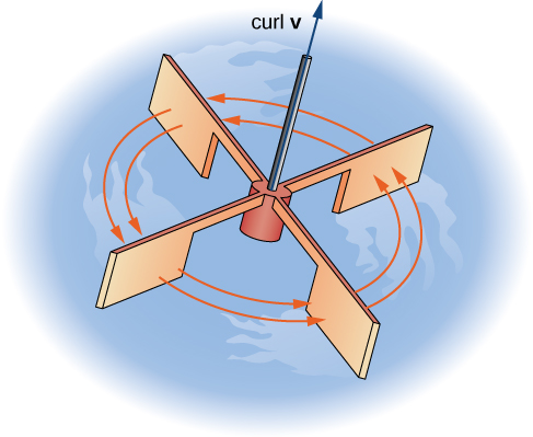
Figure 3. To visualize curl at a point, imagine placing a tiny paddlewheel at that point in the vector field.
Now that we have learned about Stokes’ theorem, we can discuss applications in the area of electromagnetism. In particular, we examine how we can use Stokes’ theorem to translate between two equivalent forms of Faraday’s law. Before stating the two forms of Faraday’s law, we need some background terminology.
Let [latex]C[/latex] be a closed curve that models a thin wire. In the context of electric fields, the wire may be moving over time, so we write [latex]C(t)[/latex] to represent the wire. At a given time [latex]t[/latex], curve [latex]C(t)[/latex] may be different from original curve [latex]C[/latex] because of the movement of the wire, but we assume that [latex]C(t)[/latex] is a closed curve for all times [latex]t[/latex]. Let [latex]D(t)[/latex] be a surface with [latex]C(t)[/latex] as its boundary, and orient [latex]C(t)[/latex] so that [latex]D(t)[/latex] has positive orientation. Suppose that [latex]C(t)[/latex] is in a magnetic field [latex]{\bf{B}}(t)[/latex] that can also change over time. In other words, [latex]{\bf{b}}[/latex] has the form
[latex]\large{{\bf{B}}(x,y,z)=\langle{P}(x,y,z),Q(x,y,z),R(x,y,z)\rangle}[/latex],
where [latex]P[/latex], [latex]Q[/latex], and [latex]R[/latex] can all vary continuously over time. We can produce current along the wire by changing field [latex]{\bf{B}}(t)[/latex] (this is a consequence of Ampere’s law). Flux [latex]\phi(t)=\displaystyle\iint_{D(t)}{\bf{B}}(t)\cdot{d}{\bf{S}}[/latex] creates electric field [latex]{\bf{E}}(t)[/latex] that does work. The integral form of Faraday’s law states that
[latex]\large{\text{Work }=\displaystyle\int_{C(t)}{\bf{E}}(t)\cdot{d}{\bf{r}}=-\frac{\partial\phi}{\partial{t}}}[/latex].
In other words, the work done by [latex]{\bf{E}}[/latex] is the line integral around the boundary, which is also equal to the rate of change of the flux with respect to time. The differential form of Faraday’s law states that
[latex]\large{\text{curl }{\bf{E}}=-\frac{\partial{\bf{B}}}{\partial{t}}}[/latex].
Using Stokes’ theorem, we can show that the differential form of Faraday’s law is a consequence of the integral form. By Stokes’ theorem, we can convert the line integral in the integral form into surface integral
[latex]\large{-\frac{\partial\phi}{\partial{t}}=\displaystyle\int_{C(t)}{\bf{E}}(t)\cdot{d}{\bf{r}}=\displaystyle\iint_{D(t)}\text{curl }{\bf{E}}(t)\cdot{d}{\bf{S}}}[/latex].
Since [latex]\phi(t)=\displaystyle\iint_{D(t)}{\bf{B}}(t)\cdot{d}{\bf{S}}[/latex], then as long as the integration of the surface does not vary with time we also have
[latex]\large{-\frac{\partial\phi}{\partial{t}}=\displaystyle\iint_{D(t)}-\frac{\partial{\bf{B}}}{\partial{t}}\cdot{d}{\bf{S}}}[/latex].
Therefore,
[latex]\large{\displaystyle\iint_{D(t)}-\frac{\partial{\bf{B}}}{\partial{t}}\cdot{d}{\bf{S}}=\displaystyle\iint_{D(t)}\text{curl }{\bf{E}}(t)\cdot{d}{\bf{S}}}[/latex].
To derive the differential form of Faraday’s law, we would like to conclude that [latex]\text{curl }{\bf{E}}=-\frac{\partial{\bf{B}}}{\partial{t}}[/latex]. In general, the equation
[latex]large{\displaystyle\iint_{D(t)}-\frac{\partial{\bf{B}}}{\partial{t}}\cdot{d}{\bf{S}}=\displaystyle\iint_{D(t)}\text{curl }{\bf{E}}(t)\cdot{d}{\bf{S}}}[/latex]
is not enough to conclude that [latex]\text{curl }{\bf{E}}=-\frac{\partial{\bf{B}}}{\partial{t}}[/latex]. The integral symbols do not simply “cancel out,” leaving equality of the integrands. To see why the integral symbol does not just cancel out in general, consider the two single-variable integrals [latex]\displaystyle\int_0^1xdx[/latex] and [latex]\displaystyle\int_0^1f(x)dx[/latex], where
[latex]f(x)=\begin{array}{cc} \{ & \begin{array}{cc} 1, & 0\leq{x}\leq1/2 \\ 0,& 1/2\leq{x}\leq1 \end{array} \end{array}[/latex].
Both of these integrals equal [latex]\frac12[/latex], so[latex]\displaystyle\int_0^1xdx=\displaystyle\int_0^1f(x)dx[/latex]. However, [latex]x\ne{f}(x)[/latex]. Analogously, with our equation [latex]\displaystyle\iint_{D(t)}-\frac{\partial{\bf{B}}}{\partial{t}}\cdot{d}{\bf{S}}=\displaystyle\iint_{D(t)}\text{curl }{\bf{E}}(t)\cdot{d}{\bf{S}}[/latex], we cannot simply conclude that [latex]\text{curl }{\bf{E}}=-\frac{\partial{\bf{B}}}{\partial{t}}[/latex] just because their integrals are equal. However, in our context, equation [latex]\displaystyle\iint_{D(t)}-\frac{\partial{\bf{B}}}{\partial{t}}\cdot{d}{\bf{S}}=\displaystyle\iint_{D(t)}\text{curl }{\bf{E}}(t)\cdot{d}{\bf{S}}[/latex] is true for any region, however small (this is in contrast to the single-variable integrals just discussed). If [latex]{\bf{F}}[/latex] and [latex]{\bf{G}}[/latex] are three-dimensional vector fields such that [latex]\displaystyle\iint_S{\bf{F}}\cdot{d}{\bf{S}}=\displaystyle\iint_S{\bf{G}}\cdot{d}{\bf{S}}[/latex] for any surface [latex]S[/latex], then it is possible to show that [latex]{\bf{F}}={\bf{G}}[/latex] by shrinking the area of [latex]S[/latex] to zero by taking a limit (the smaller the area of [latex]S[/latex], the closer the value of [latex]\displaystyle\iint_S{\bf{F}}\cdot{d}{\bf{S}}[/latex] to the value of [latex]{\bf{F}}[/latex] at a point inside [latex]S[/latex]). Therefore, we can let area [latex]D(t)[/latex] shrink to zero by taking a limit and obtain the differential form of Faraday’s law:
[latex]\large{\text{curl }{\bf{E}}=-\frac{\partial{\bf{B}}}{\partial{t}}}[/latex].
In the context of electric fields, the curl of the electric field can be interpreted as the negative of the rate of change of the corresponding magnetic field with respect to time.
Example: Using Faraday’s law
Calculate the curl of electric field [latex]{\bf{E}}[/latex] if the corresponding magnetic field is constant field [latex]{\bf{B}}(t)=\langle1,-4,2\rangle[/latex].
try it
Calculate the curl of electric field [latex]{\bf{E}}[/latex] if the corresponding magnetic field is [latex]{\bf{B}}(t)=\langle{t}x,ty,-2tz\rangle[/latex], [latex]0\leq{t}<\infty[/latex].
Notice that the curl of the electric field does not change over time, although the magnetic field does change over time.
Watch the following video to see the worked solution to the above Try It
Candela Citations
- CP 6.63. Authored by: Ryan Melton. License: CC BY: Attribution
- CP 6.64. Authored by: Ryan Melton. License: CC BY: Attribution
- Calculus Volume 3. Authored by: Gilbert Strang, Edwin (Jed) Herman. Provided by: OpenStax. Located at: https://openstax.org/books/calculus-volume-3/pages/1-introduction. License: CC BY-NC-SA: Attribution-NonCommercial-ShareAlike. License Terms: Access for free at https://openstax.org/books/calculus-volume-3/pages/1-introduction
