The right-hand side of the Directional Derivative of a Function of Two Variables is equal to [latex]f_x(x,y)\cos\theta+f_y(x,y)\sin\theta[/latex], which can be written as the dot product of two vectors. Define the first vector as [latex]\nabla{f}(x,y)=f_x(x,y){\bf{i}}+f_y(x,y)\bf{j}[/latex] and the second vector as [latex]{\bf{u}}=(\cos\theta){\bf{i}}+(\sin\theta)\bf{j}[/latex]. Then the right-hand side of the equation can be written as the dot product of these two vectors:

[latex]D_{\bf{u}}f(x,y)=\nabla{f}(x,y)\cdot\bf{u}.[/latex]

The first vector in the previous equation has a special name: the gradient of the function [latex]f[/latex]. The symbol [latex]\nabla[/latex] is called nabla and the vector [latex]\nabla{f}[/latex] is read “del [latex]f[/latex]“.

The gradient has some important properties. We have already seen one formula that uses the gradient: the formula for the directional derivative. Recall from The Dot Product that if the angle between two vectors [latex]\bf{a}[/latex] and [latex]\bf{b}[/latex] is [latex]\varphi[/latex], then [latex]{\bf{a}}\cdot{\bf{b}}=\|{\bf{a}}\|\|{\bf{b}}\|\cos\varphi[/latex]. Therefore, if the angle between [latex]\nabla{f}(x_0,y_0)[/latex] and [latex]{\bf{u}}=(\cos\theta){\bf{i}}+(\sin\theta){\bf{j}}[/latex] is [latex]\varphi[/latex], we have

[latex]\large{D_{\bf{u}}f(x_0,y_0)=\nabla{f}(x_0,y_0)\cdot{\bf{u}}=\|\nabla{f}(x_0,y_0)\|\|{\bf{u}}\|\cos\varphi=\|\nabla{f}(x_0,y_0)\|\cos\varphi}[/latex]

The [latex]\|{\bf{u}}\|[/latex] disappears because [latex]\bf{u}[/latex] is a unit vector. Therefore, the directional derivative is equal to the magnitude of the gradient evaluated at [latex](x_0, y_0)[/latex], multiplied by [latex]\cos\varphi[/latex]. Recall that [latex]\cos\varphi[/latex] ranges from [latex]-1[/latex] to [latex]1[/latex]. If [latex]\varphi=0[/latex], then [latex]\cos\varphi=1[/latex] and [latex]\nabla{f}(x_0,y_0)[/latex] and [latex]\bf{u}[/latex] point in opposite directions. In the first case, the value of [latex]D_{\bf{u}}f(x_0,y_0)[/latex] is maximized; in the second case, the value of [latex]D_{\bf{u}}f(x_0,y_0)[/latex] is minimized. If [latex]\nabla{f}(x_0,y_0)=0[/latex], then [latex]D_{\bf{u}}f(x_0,y_0)=\nabla{f}(x_0,y_0)\cdot{\bf{u}}=0[/latex] for any vector [latex]\bf{u}[/latex]. These cases are outlined in the following theorem.

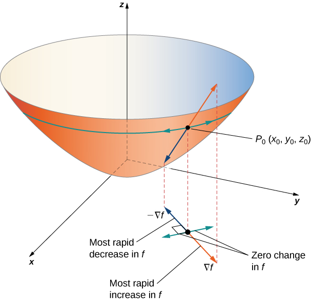
Figure 1. The gradient indicates the maximum and minimum values of the directional derivative at a point.

Example: finding a maximum directional derivative

Find the direction for which the directional derivative of [latex]f(x, y)=3x^{2}-4xy+2y^{2}[/latex] at [latex](-2, 3)[/latex] is a maximum. What is the maximum value?

Show Solution

The maximum value of the directional derivative occurs when [latex]\nabla{f}[/latex] and the unit vector point in the same direction. Therefore, we start by calculating [latex]\nabla{f}(x,y)[/latex]:

[latex]\hspace{6cm}\large{\begin{align} f_x(x,y)&=6x-4y\text{ and }f_y(x,y)=-4x+4y,\text{ so} \\ \nabla{f}(x,y)&=f_x(x,y){\bf{i}}+f_y(x,y){\bf{j}}=(6x-4y){\bf{i}}+(-4x+4y){\bf{j}}. \end{align}}[/latex]

Next, we evaluate the gradient at [latex](-2,3)[/latex]:

[latex]\large{\nabla{f}(-2,3)=(6(-2)-4(3)){\bf{i}}+(-4(-2)+3(3)){\bf{j}}=-24{\bf{i}}+20{\bf{j}}}.[/latex]

We need to find a unit vector that points in the same direction as [latex]\nabla{f}(-2,3)[/latex], so the next step is to divide [latex]\nabla{f}(-2,3)[/latex] by its magnitude, which is [latex]\sqrt{(-24)^2+(20)^2}=\sqrt{976}=4\sqrt{61}[/latex]. Therefore,

[latex]\large{\frac{\nabla{f}(-2,3)}{\|\nabla{f}(-2,3)\|}=\frac{-24}{4\sqrt{61}}{\bf{i}}+\frac{20}{4\sqrt{61}}{\bf{j}}=\frac{-6\sqrt{61}}{61}{\bf{i}}+\frac{5\sqrt{61}}{61}{\bf{j}}}.[/latex]

This is the unit vector that points in the same direction as [latex]\nabla{f}(-2,3)[/latex]. To find the angle corresponding to this unit vector, we solve the equations

[latex]\large{\cos\theta=\frac{-6\sqrt{61}}{61}}[/latex] and [latex]\large{\sin\theta=\frac{5\sqrt{61}}{61}}.[/latex]

for [latex]\theta[/latex]. Since cosine is negative and sine is positive, the angle must be in the second quadrant. Therefore,

[latex]\theta=\pi-\arcsin{((5\sqrt{61})/61)}\approx2.45\text{ rad}.[/latex]

The maximum value of the directional derivative at [latex](-2, 3)[/latex] is [latex]\|\nabla{f}(-2,3)\|=4\sqrt{61}[/latex] (see the following figure).

Figure 2. The maximum value of the directional derivative at [latex]\small{(-2,3)}[/latex] is in the direction of the gradient.

Watch the following video to see the worked solution to the above Try It

.

Figure 5 shows a portion of the graph of the function [latex]f(x,y)=3+\sin x\sin y[/latex]. Given a point [latex](a, b)[/latex] in the domain of [latex]f[/latex], the maximum value of the gradient at that point is given by [latex]\|\nabla{f}(a,b)\|[/latex]. This would equal the rate of greatest ascent if the surface represented a topographical map. If we went in the opposite direction, it would be the rate of greatest descent.

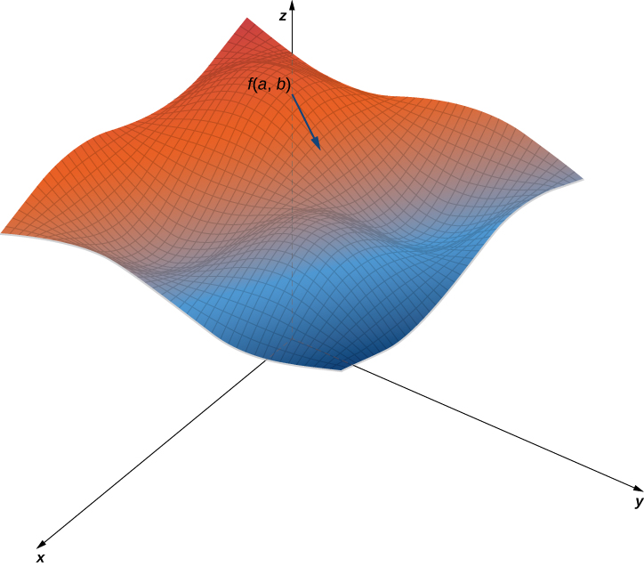
Figure 3. A typical surface in [latex]\mathbb{R}^{3}[/latex]. Given a point on the surface, the directional derivative can be calculated using the gradient.

When using a topographical map, the steepest slope is always in the direction where the contour lines are closest together (see Figure 6). This is analogous to the contour map of a function, assuming the level curves are obtained for equally spaced values throughout the range of that function.

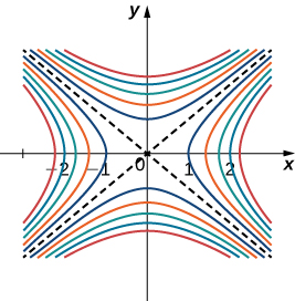
Figure 4. Contour map for the function [latex]\small{f(x,y)=x^{2}-y^{2}}[/latex] using level values between [latex]\small{-5}[/latex] and [latex]\small{5}[/latex].

Gradients and Level Curves

Recall that if a curve is defined parametrically by the function pair [latex](x(t), y(t))[/latex], then the vector [latex]x'(t){\bf{i}}+y'(t){\bf{j}}[/latex] is tangent to the curve for every value of [latex]t[/latex] in the domain. Now let’s assume [latex]z=f(x, y)[/latex] is a differentiable function of [latex]x[/latex] and [latex]y[/latex], and [latex](x_0, y_0)[/latex] is in its domain. Let’s suppose further that [latex]x_0=x(t_0)[/latex] and [latex]y_0=y(t_0)[/latex] for some value of [latex]t[/latex], and consider the level curve [latex]f(x, y)=k[/latex]. Define [latex]g(t)=f(x(t), y(t))[/latex] and calculate [latex]{g}'(t)[/latex] on the level curve. By the Chain Rule,

[latex]\large{g'(t)=f_x(x(t),y(t))x'(t)+f_y(x(t),y(t))y'(t)}.[/latex]

But [latex]g'(t)=0[/latex] because [latex]g(t)=k[/latex] for all [latex]t[/latex]. Therefore, on the one hand,

[latex]\large{f_x(x(t),y(t))x'(t)+f_y(x(t),y(t))y'(t)=0};[/latex]

on the other hand,

[latex]\large{f_x(x(t),y(t))x'(t)+f_y(x(t),y(t))y'(t)=\nabla{f}(x,y)\cdot\langle{x}'(t),y'(t)\rangle}.[/latex]

Therefore,

[latex]\large{\nabla{f}(x,y)\cdot\langle{x}'(t),y'(t)\rangle=0}.[/latex]

Thus, the dot product of these vectors is equal to zero, which implies they are orthogonal. However, the second vector is tangent to the level curve, which implies the gradient must be normal to the level curve, which gives rise to the following theorem.

We can use this theorem to find tangent and normal vectors to level curves of a function.

Example: Finding Tangents to level curves

For the function [latex]f(x, y)=2x^{2}-3xy+8y^{2}+2x-4y+4[/latex], find a tangent vector to the level curve at point [latex](-2, 1)[/latex]. Graph the level curve corresponding to [latex]f(x, y)=18[/latex] and draw in [latex]\nabla{f}(-2,1)[/latex] and a tangent vector.

Show Solution

First, we must calculate [latex]\nabla{f}(x,y)[/latex]:

[latex]f_x(x,y)=4x-3y+2[/latex] and [latex]f_y=-3x+16y-4[/latex] so [latex]\nabla{f}(x,y)=(4x-3y+2){\bf{i}}+(-3x+16y-4){\bf{j}}.[/latex]

Next, we evaluate [latex]\nabla{f}(x,y)[/latex] at [latex](-2,1)[/latex]:

[latex]\nabla{f}(-2,1)=(4(-2)-3(1)+2){\bf{i}}+(-3(-2)+16(1)-4){\bf{j}}=-9{\bf{i}}+18{\bf{j}}.[/latex]

This vector is orthogonal to the curve at point [latex](-2, 1)[/latex]. We can obtain a tangent vector by reversing the components and multiplying either one by [latex]-1[/latex]. Thus, for example, [latex]-18{\bf{i}}-9{\bf{j}}[/latex] is a tangent vector (see the following graph).

Figure 5. A rotated ellipse with equation [latex]\small{f(x,y)=18}[/latex]. At the point [latex]\small{(-2,1)}[/latex] on the ellipse, there are drawn two arrows, one tangent vector and one normal vector. The normal vector is marked [latex]\small{\nabla{f(-2,1)}}[/latex] and is perpendicular to the tangent vector.

Try it

For the function [latex]f(x,y)=x^2-2xy+5y^2+3x-2y+4[/latex], find the tangent to the level curve at point [latex](1, 1)[/latex]. Draw the graph of the level curve corresponding to [latex]f(x, y)=8[/latex] and draw [latex]\nabla{f}(1,1)[/latex] and a tangent vector.

Show Solution

[latex]\nabla{f}(x,y)=(2x-2y+3){\bf{i}}+(-2x+10y-2){\bf{j}}[/latex]

[latex]\nabla{f}(1,1)=3{\bf{i}}+6{\bf{j}}[/latex]

Tangent vector: [latex]6{\bf{i}}-6{\bf{j}}[/latex] or [latex]-6{\bf{i}}+3{\bf{j}}[/latex]

Figure 6.