Learning Outcomes
- Calculate the limit of a function of two variables.
- Learn how a function of two variables can approach different values at a boundary point, depending on the path of approach.
Recall from The Limit of a Function the definition of a limit of a function of one variable:
Let [latex]f\,(x)[/latex] be defined for all [latex]x\neq{a}[/latex] in an open interval containing [latex]a[/latex]. Let [latex]L[/latex] be a real number. Then
[latex]\displaystyle{\lim_{x\to{a}}}f\,(x)=L[/latex]
if for every [latex]\epsilon\,>\,0[/latex], there exists a [latex]\delta\,>\,0[/latex], such that if [latex]0\,<\,|x-a|\,<\delta[/latex] for all [latex]x[/latex] in the domain of [latex]f[/latex], then
[latex]|f\,(x)-L|\,<\,\epsilon[/latex]
Before we can adapt this definition to define a limit of a function of two variables, we first need to see how to extend the idea of an open interval in one variable to an open interval in two variables.
Definition
Consider a point [latex](a,\ b)\in\mathbb{R}^2[/latex]. A [latex]\delta[/latex] disk centered at point [latex](a,\ b)[/latex] is defined to be an open disk of radius [latex]\delta[/latex] centered at point [latex](a,\ b)[/latex] – that is,
[latex]\{(x,\ y)\in\mathbb{R}^{2}|(x-a)^{2}+(y-b)^{2}<\,\delta^{2}\}[/latex]
as shown in the following graph.
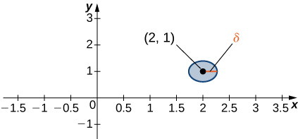
Figure 1. A [latex]\delta[/latex] disk centered around the point [latex](2,1)[/latex].
The idea of a [latex]\delta[/latex] disk appears in the definition of the limit of a function of two variables. If [latex]\delta[/latex] is small, then all the points [latex](x,\ y)[/latex] in the [latex]\delta[/latex] disk are close to [latex](a,\ b)[/latex]. This is completely analogous to [latex]x[/latex] being close to [latex]a[/latex] in the definition of a limit of a function of one variable. In one dimension, we express this restriction as
[latex]a-\delta\,<\,x\,<\,a+\delta[/latex].
In more than one dimension, we use a [latex]\delta[/latex] disk.
Definition
Let [latex]f[/latex] be a function of two variables, [latex]x[/latex] and [latex]y[/latex]. The limit of [latex]f\,(x,\ y)[/latex] as [latex](x,\ y)[/latex] approaches [latex](a,\ b)[/latex] is [latex]L[/latex], written
if for each [latex]\epsilon>0[/latex] there exists a small enough [latex]\delta\,>\,0[/latex] such that for all points [latex](x,\ y)[/latex] in a [latex]\delta[/latex] disk around [latex](a,\ b)[/latex], except possibly for [latex](a,\ b)[/latex] itself, the value of [latex]f\,(x,\ y)[/latex] is no more than [latex]\epsilon[/latex] away from [latex]L[/latex] (Figure 2). Using symbols, we write the following: For any [latex]\varepsilon\,>\,0[/latex], there exists a number [latex]\delta\,>\,0[/latex] such that
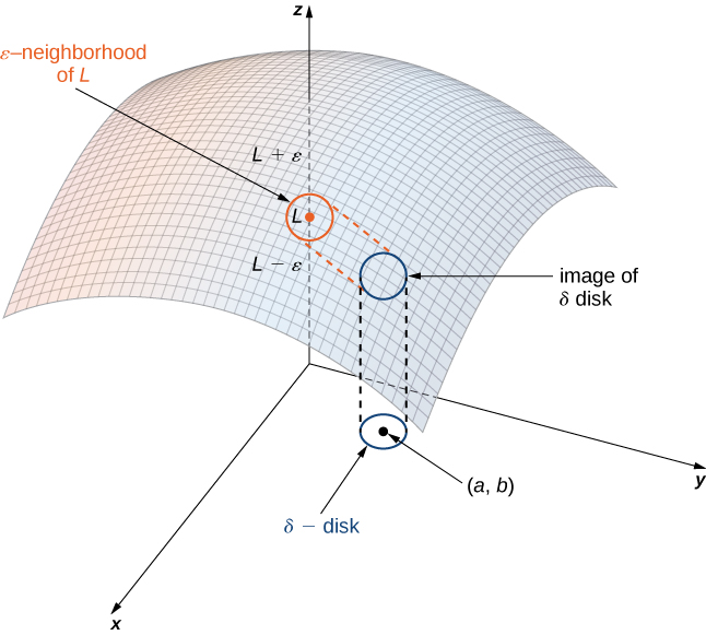
Figure 2. The limit of a function involving two variables requires that [latex]f(x,y)[/latex] be within [latex]\varepsilon[/latex] of [latex]L[/latex] whenever [latex](x,y)[/latex] is within [latex]\delta[/latex] of [latex](a,b)[/latex]. The smaller the value of [latex]\varepsilon[/latex], the smaller the value of [latex]\delta[/latex].
Proving that a limit exists using the definition of a limit of a function of two variables can be challenging. Instead, we use the following theorem, which gives us shortcuts to finding limits. The formulas in this theorem are an extension of the formulas in the limit laws theorem in The Limit Laws.
Limit LAws for Functions of Two Variables Theorem
Let [latex]f\,(x,\ y)[/latex] and [latex]g\,(x,\ y)[/latex] be defined for all [latex](x,\ y)\neq(a,\ b)[/latex] in a neighborhood around [latex](a,\ b)[/latex], and assume the neighborhood is contained completely inside the domain of [latex]f[/latex]. Assume that [latex]L[/latex] and [latex]M[/latex] are real numbers such that [latex]\displaystyle\lim_{(x,\ y)\to(a,\ b)}f\,(x,\ y)=L[/latex] and [latex]\displaystyle\lim_{(x,\ y)\to(a,\ b)}g\,(x,\ y)=M[/latex], and let [latex]c[/latex] be a constant. Then each of the following statements holds:
Constant Law:
[latex]\displaystyle\lim_{(x,\ y)\to(a,\ b)}c=c[/latex]
Identity Law:
[latex]\begin{array}{ccc}\hfill {\displaystyle\lim_{(x,\ y)\to(a,\ b)}x} & =\hfill & {a} \hfill \\ \hfill {\displaystyle\lim_{(x,\ y)\to(a,\ b)}y} & =\hfill & {b} \end{array}[/latex]
Sum Law:
[latex]\displaystyle\lim_{(x,\ y)\to(a,\ b)}(f\,(x,\ y)+g\,(x,\ y))=L+M[/latex]
Difference Law:
[latex]\displaystyle\lim_{(x,\ y)\to(a,\ b)}(f\,(x,\ y)-(g\,(x,\ y))=L-M[/latex]
Constant Multiple Law:
[latex]\displaystyle\lim_{(x,\ y)\to(a,\ b)}(cf\,(x,\ y))=cL[/latex]
Product Law:
[latex]\displaystyle\lim_{(x,\ y)\to(a,\ b)}(f\,(x,\ y)\,g\,(x,\ y))=LM[/latex]
Quotient Law:
[latex]\displaystyle\lim_{(x,\ y)\to(a,\ b)}\frac{f\,(x,\ y)}{g\,(x,\ y)}=\frac{L}{M}[/latex] for [latex]M\neq{0}[/latex]
Power Law:
[latex]\displaystyle\lim_{(x,\ y)\to(a,\ b)}(f\,(x,\ y))^{n}=L^{n}[/latex]
for any positive integer [latex]n[/latex].
Root Law:
[latex]\displaystyle\lim_{(x,\ y)\to(a,\ b)}\sqrt[n]{f\,(x,\ y)}=\sqrt[n]{L}[/latex]
for all [latex]L[/latex] if [latex]n[/latex] is odd and positive, and for [latex]L\,\geq\,0[/latex] if [latex]n[/latex] is even and positive.
The proofs of these properties are similar to those for the limits of functions of one variable. We can apply these laws to finding limits of various functions.
Example: Finding the Limit of a Function of Two Variables
Find each of the following limits:
- [latex]\displaystyle\lim_{(x,\ y)\to(2,\ -1)}(x^{2}-2xy+3y^{2}-4x+3y-6)[/latex]
- [latex]\displaystyle\lim_{(x,\ y)\to(2,\ -1)}\frac{2x+3y}{4x-3y}[/latex]
Try it
Evaluate the following limit:
[latex]\displaystyle\lim_{(x,\ y)\to(5,\ -2)}\sqrt[3]{\frac{x^{2}-y}{y^{2}+x-1}.}[/latex]
Since we are taking the limit of a function of two variables, the point [latex](a,\ b)[/latex] is in [latex]\mathbb{R}^{2}[/latex], and it is possible to approach this point from an infinite number of directions. Sometimes when calculating a limit, the answer varies depending on the path taken toward [latex](a,\ b)[/latex]. If this is the case, then the limit fails to exist. In other words, the limit must be unique, regardless of path taken.
Example: Limits that Fail to Exist
Show that neither of the following limits exist:
- [latex]\displaystyle\lim_{(x,\ y)\to(0,\ 0)}\frac{2xy}{3x^{2}+y^{2}}[/latex]
- [latex]\displaystyle\lim_{(x,\ y)\to(0,\ 0)}\frac{4xy^{2}}{x^{2}+3y^{4}}[/latex]

Try it
Show that
[latex]\displaystyle\lim_{(x,\ y)\to(2,\ 1)}\frac{(x-2)(y-1)}{(x-2)^{2}+(y-1)^{2}}[/latex]
does not exist.
Watch the following video to see the worked solution to the above Try It
Interior Points and Boundary Points
To study continuity and differentiability of a function of two or more variables, we first need to learn some new terminology.
Definition
Let [latex]S[/latex] be a subset of [latex]\mathbb{R}^{2}[/latex] (Figure 4).
- A point [latex]P_0[/latex] is called an interior point of [latex]S[/latex] if there is a [latex]\delta[/latex] disk centered around [latex]P_0[/latex] contained completely in [latex]S[/latex].
- A point [latex]P_0[/latex] is called a boundary point of [latex]S[/latex] if every [latex]\delta[/latex] disk centered around [latex]P_0[/latex] contains points both inside and outside [latex]S[/latex].
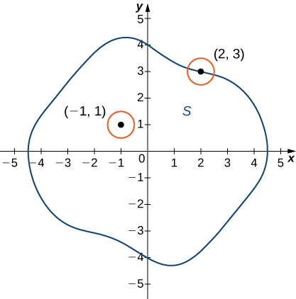
Figure 4. In the set [latex]S[/latex] shown, [latex]\small{(-1,1)}[/latex] is an interior point and [latex]\small{(2,3)}[/latex] is a boundary point.
Definition
Let [latex]S[/latex] be a subset of [latex]\mathbb{R}^{2}[/latex] (Figure 4).
- [latex]S[/latex] is called an open set if every point of [latex]S[/latex] is an interior point.
- [latex]S[/latex] is called a closed set if it contains all its boundary points.
An example of an open set is a [latex]\delta[/latex] disk. If we include the boundary of the disk, then it becomes a closed set. A set that contains some, but not all, of its boundary points is neither open nor closed. For example if we include half the boundary of a [latex]\delta[/latex] disk but not the other half, then the set is neither open nor closed.
Definition
Let [latex]S[/latex] be a subset of [latex]\mathbb{R}^{2}[/latex] (Figure 4).
- An open set [latex]S[/latex] is a connected set if it cannot be represented as the union of two or more disjoint, nonempty open subsets.
- A set [latex]S[/latex] is a region if it is open, connected, and nonempty.
The definition of a limit of a function of two variables requires the [latex]\delta[/latex] disk to be contained inside the domain of the function. However, if we wish to find the limit of a function at a boundary point of the domain, the [latex]\delta[/latex] disk is not contained inside the domain. By definition, some of the points of the [latex]\delta[/latex] disk are inside the domain and some are outside. Therefore, we need only consider points that are inside both the [latex]\delta[/latex] disk and the domain of the function. This leads to the definition of the limit of a function at a boundary point.
Definition
Let [latex]f[/latex] be a function of two variables, [latex]x[/latex] and [latex]y[/latex], and suppose [latex](a,\ b)[/latex] is on the boundary of the domain of [latex]f[/latex]. Then, the limit of [latex]f\,(x,\ y)[/latex] as [latex](x,\ y)[/latex] approaches [latex](a,\ b)[/latex] is [latex]L[/latex], written
if for any [latex]\epsilon\,>\,0[/latex], there exists a number [latex]\delta\,>\,0[/latex] such that for any point [latex](x,\ y)[/latex] inside the domain of [latex]f[/latex] and within a suitably small distance positive [latex]\delta[/latex] of [latex](a,\ b)[/latex], the value of [latex]f\,(x,\ y)[/latex] is no more than [latex]\epsilon[/latex] away from [latex]L[/latex] (Figure 2). Using symbols, we can write: For any [latex]\epsilon\,>\,0[/latex], there exists a number [latex]\delta\,>\,0[/latex] such that
Example: Limit of a Function at a Boundary Point
Prove [latex]\displaystyle\lim_{(x,\ y)\to(4,\ 3)}\sqrt{25-x^{2}-y^{2}}=0[/latex].


Try it
Evaluate the following limit:
[latex]\displaystyle\lim_{(x,\ y)\to(5,-2)}\sqrt{29-x^{2}-y^{2}}.[/latex]
Watch the following video to see the worked solution to the above Try It
Candela Citations
- CP 4.7. Authored by: Ryan Melton. License: CC BY: Attribution
- CP 4.8. Authored by: Ryan Melton. License: CC BY: Attribution
- Calculus Volume 3. Authored by: Gilbert Strang, Edwin (Jed) Herman. Provided by: OpenStax. Located at: https://openstax.org/books/calculus-volume-3/pages/1-introduction. License: CC BY-NC-SA: Attribution-NonCommercial-ShareAlike. License Terms: Access for free at https://openstax.org/books/calculus-volume-3/pages/1-introduction
