Learning Outcomes
- State Kepler’s laws of planetary motion.
Now let’s look at an application of vector functions. In particular, let’s consider the effect of gravity on the motion of an object as it travels through the air, and how it determines the resulting trajectory of that object. In the following, we ignore the effect of air resistance. This situation, with an object moving with an initial velocity but with no forces acting on it other than gravity, is known as projectile motion. It describes the motion of objects from golf balls to baseballs, and from arrows to cannonballs.
First we need to choose a coordinate system. If we are standing at the origin of this coordinate system, then we choose the positive y-axis to be up, the negative y-axis to be down, and the positive x-axis to be forward (i.e., away from the thrower of the object). The effect of gravity is in a downward direction, so Newton’s second law tells us that the force on the object resulting from gravity is equal to the mass of the object times the acceleration resulting from to gravity, or [latex]F_{g}=mg[/latex], where [latex]F_{g}[/latex] represents the force from gravity and [latex]g[/latex] represents the acceleration resulting from gravity at Earth’s surface. The value of [latex]g[/latex] in the English system of measurement is approximately [latex]32\ ft/sec^{2}[/latex] and it is approximately [latex]9.8\ m/sec^{2}[/latex] in the metric system. This is the only force acting on the object. Since gravity acts in a downward direction, we can write the force resulting from gravity in the form [latex]F_{g}=-mg\,{\bf{j}}[/latex], as shown in the following figure.
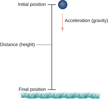
Figure 1. An object is falling under the influence of gravity.
Interactive
Visit this website for a video showing projectile motion.
Newton’s second law also tells us that [latex]F=m{\bf{a}}[/latex], where [latex]\bf{a}[/latex] represents the acceleration vector of the object. This force must be equal to the force of gravity at all times, so we therefore know that
[latex]\begin{array}{ccc}\hfill {F} & =\hfill & {F_{g}} \hfill \\ \hfill {m{\bf{a}}}& =\hfill & {-mg\,{\bf{j}}} \hfill \\ \hfill {{\bf{a}}}& =\hfill & {-g\,{\bf{j}}}\hfill \\ \hfill \end{array}[/latex]
Now we use the fact that the acceleration vector is the first derivative of the velocity vector. Therefore, we can rewrite the last equation in the form
[latex]{\bf{v}}'\,(t)=-g\,{\bf{j}}.[/latex]
By taking the antiderivative of each side of this equation we obtain
[latex]\begin{array}{ccc}\hfill {{\bf{v}}\,(t)} & =\hfill & {\displaystyle\int_{}\ -g\,{\bf{j}}\,dt} \hfill \\ \hfill & =\hfill & {-gt\,{\bf{j}}+{\bf{C}}_{1}}\hfill \\ \hfill \end{array}[/latex]
for some constant vector [latex]{\bf{C}}_{1}[/latex]. To determine the value of this vector, we can use the velocity of the object at a fixed time, say at time [latex]t=0[/latex]. We call this velocity the initial velocity: [latex]{\bf{v}}\,(0)={\bf{v}}_{0}[/latex]. Therefore, [latex]{\bf{v}}\,(0)=-g\,(0)\,{\bf{j}}+{\bf{C}}_{1}={\bf{v}}_{0}[/latex] and [latex]{\bf{C}}_{1}={\bf{v}}_{0}[/latex]. This gives the velocity vector as [latex]{\bf{v}}\,(t)=-gt\,{\bf{j}}+{\bf{v}}_{0}[/latex].
Next we use the fact that velocity [latex]{\bf{v}}\,(t)[/latex] is the derivative of position [latex]{\bf{s}}\,(t)[/latex]. This gives the equation
[latex]{\bf{s}}'\,(t)=-gt\,{\bf{j}}+{\bf{v}}_{0}[/latex].
Taking the antiderivative of both sides of this equation leads to
[latex]\begin{array}{ccc}\hfill {{\bf{s}}\,(t)} & =\hfill & {\displaystyle\int_{}\ -gt\,{\bf{j}}+{\bf{v}}_{0}\,dt} \hfill \\ \hfill & =\hfill & {-\frac{1}{2}\,gt^{2}\,{\bf{j}}+{\bf{v}}_{0}t+{\bf{C}}_{2},}\hfill \\ \hfill \end{array}[/latex]
with another unknown constant vector [latex]{\bf{C}}_{2}[/latex]. To determine the value of [latex]{\bf{C}}_{2}[/latex], we can use the position of the object at a given time, say at time [latex]t=0[/latex]. We call this position the initial position: [latex]{\bf{s}}\,(0)={\bf{s}}_{0}[/latex]. Therefore, [latex]{\bf{s}}\,(0)=-(1/2)\,g(0)^{2}\,{\bf{j}}+{\bf{v}}_{0}\,(0)+{\bf{C}}_{2}={\bf{s}}_{0}[/latex] and [latex]{\bf{C}}_{2}={\bf{s}}_{0}[/latex]. This gives the position of the object at any time as
[latex]{\bf{s}}\,(t)=-\frac{1}{2}\,gt^{2}\,{\bf{j}}+{\bf{v}}_{0}\,t+{\bf{s}}_{0}.[/latex]
Let’s take a closer look at the initial velocity and initial position. In particular, suppose the object is thrown upward from the origin at an angle [latex]\theta[/latex] to the horizontal, with initial speed [latex]v_{0}[/latex]. How can we modify the previous result to reflect this scenario? First, we can assume it is thrown from the origin. If not, then we can move the origin to the point from where it is thrown. Therefore, [latex]{\bf{s}}_{0}={\bf{0}}[/latex], as shown in the following figure.
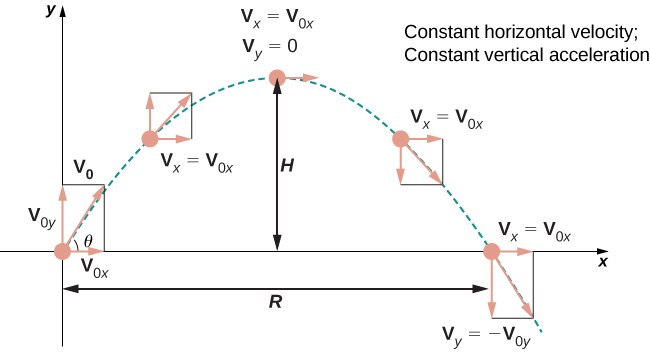
Figure 2. Projectile motion when the object is thrown upward at an angle [latex]\theta[/latex]. The horizontal motion is at constant velocity and the vertical motion is at constant acceleration.
We can rewrite the initial velocity vector in the form [latex]{\bf{v}}_{0}=v_{0}\cos{\theta}{\bf{i}}+v_{0}\sin{\theta}{\bf{j}}[/latex]. Then the equation for the position functions [latex]{\bf{s}}(t)[/latex] becomes
[latex]\begin{array}{ccc}\hfill {{\bf{s}}\,(t)} & =\hfill & {-\frac{1}{2}gt^{2}{\bf{j}}+v_{0}t\cos{\theta{\bf{i}}}+v_{0}t\sin{\theta{\bf{j}}}} \hfill \\ \hfill & =\hfill & {v_{0}t\cos{\theta{\bf{i}}}+v_{0}t\sin{\theta{\bf{j}}}-\frac{1}{2}gt^{2}\,{\bf{j}}}\hfill \\ \hfill & =\hfill & {v_{0}t\cos{\theta{\bf{i}}}+(v_{0}t\sin{\theta}-\frac{1}{2}gt^{2})\,{\bf{j}}.}\hfill \\ \hfill \end{array}[/latex]
The coefficient of [latex]{\bf{i}}[/latex] represents the horizontal component of [latex]{\bf{s}}(t)[/latex] and is the horizontal distance of the object from the origin at time [latex]t[/latex]. The maximum value of the horizontal distance (measured at the same initial and final attitude) is called the range [latex]R[/latex]. The coefficient of [latex]{\bf{j}}[/latex] represents the vertical component of [latex]{\bf{s}}(t)[/latex] and is the altitude of the object at time [latex]t[/latex]. The maximum value of the vertical distance is the height [latex]H[/latex].
Example: Motion of a Cannonball
During an Independence Day celebration, a cannonball is fired from a cannon on a cliff toward the water. The cannon is aimed at an angle of [latex]30^\circ[/latex] above horizontal and the initial speed of the cannonball is [latex]600\ ft/sec[/latex]. The cliff is [latex]100\ ft[/latex] above the water (Figure 7).
- Find the maximum height of the cannonball.
- How long will it take for the cannonball to splash into the sea?
- How far out to sea will the cannonball hit the water?

Figure 3. The flight of a cannonball (ignoring air resistance) is projectile motion.
try it
An archer fires an arrow at an angle of [latex]40^\circ[/latex] above the horizontal with an initial speed of [latex]98\text{ }m/sec[/latex]. The height of the archer is [latex]171.5\text{ }cm[/latex]. Find the horizontal distance the arrow travels before it hits the ground.
Watch the following video to see the worked solution to the above Try It
One final question remains: In general, what is the maximum distance a projectile can travel, given its initial speed? To determine this distance, we assume the projectile is fired from ground level and we wish it to return to ground level. In other words, we want to determine an equation for the range. In this case, the equation of projectile motion is
[latex]{\bf{s}}(t)=v_{0}t\cos{\theta{\bf{i}}}+(v_{0}t\sin{\theta}-\frac{1}{2}gt^{2})\,{\bf{j}}.[/latex]
Setting the second component equal to zero and solving for [latex]t[/latex] yields
[latex]\begin{array}{ccc}\hfill {v_{0}t\sin{\theta}-\frac{1}{2}gt^{2}} & =\hfill & {0} \hfill \\ \hfill {t(v_{0}\sin{\theta}-\frac{1}{2}gt)}& =\hfill & {0}\hfill \\ \hfill \end{array}[/latex]
Therefore, either [latex]t=0[/latex] or [latex]t=\frac{2v_{0}\sin{\theta}}{g}[/latex]. We are interested in the second value of [latex]t[/latex], so we substitute this into [latex]{\bf{s}}(t)[/latex], which gives
[latex]\begin{array}{ccc}\hfill{{\bf{s}}\,\big(\frac{2v_{0}\sin{\theta}}{g}\big)} & =\hfill & {v_{0}\,\big(\frac{2v_{0}\sin{\theta}}{g}\big)\cos{\theta{\bf{i}}}+\Big(v_{0}\,\big(\frac{2v_{0}\sin{\theta}}{g}\big)\sin{\theta}-\frac{1}{2}g\big(\frac{2v_{0}\sin{\theta}}{g}\big)^{2}\Big)\,{\bf{j}}} \hfill \\ \hfill & =\hfill & {\bigg(\frac{2v^2_0\sin{\theta}\cos{\theta}}{g}\bigg)\,{\bf{i}}}\hfill \\ \hfill & =\hfill & {\frac{v^2_0\sin{2\theta}}{g}\,{\bf{i}}.}\hfill \\ \hfill \end{array}[/latex]
Thus, the expression for the range of a projectile fired at an angle [latex]\theta[/latex] is
[latex]\large{R=\frac{v^2_0\sin{2\theta}}{g}\,{\bf{i}}}.[/latex]
The only variable in this expression is [latex]\theta[/latex]. To maximize the distance traveled, take the derivative of the coefficient of [latex]{\bf{i}}[/latex] with respect to [latex]\theta[/latex] and set it equal to zero:
[latex]\begin{align} \hspace{10cm} \frac{d}{d\theta}\left(\frac{v_{0}^2t\sin{2\theta}}{g}\right) & =0 \\ \frac{2v_{0}\cos{2\theta}}{g} & = 0 \\ \theta & = 45^\circ. \end{align}[/latex]
This value of [latex]\theta[/latex] is the smallest positive value that makes the derivative equal to zero. Therefore, in the absence of air resistance, the best angle to fire a projectile (to maximize the range) is at a [latex]45^\circ[/latex] angle. The distance it travels is given by
[latex]\large{{\bf{s}}\bigg(\frac{2v_{0}\sin{45}}{g}\bigg)=\frac{v^2_0\sin{90}}{g}\,{\bf{i}}=\frac{v^2_0}{g}\,{\bf{j}}}.[/latex]
Therefore, the range for an angle of [latex]45^\circ[/latex] is [latex]v^2_0/g[/latex].
Kepler’s Laws
During the early 1600s, Johannes Kepler was able to use the amazingly accurate data from his mentor Tycho Braheto formulate his three laws of planetary motion, now known as Kepler’s laws of planetary motion. These laws also apply to other objects in the solar system in orbit around the Sun, such as comets (e.g., Halley’s comet) and asteroids. Variations of these laws apply to satellites in orbit around Earth.
Kepler’s Laws of Planetary Motion Theorem
- The path of any planet about the Sun is elliptical in shape, with the center of the Sun located at one focus of the ellipse (the law of ellipses).
- A line drawn from the center of the Sun to the center of a planet sweeps out equal areas in equal time intervals (the law of equal areas) (Figure 8).
- The ratio of the squares of the periods of any two planets is equal to the ratio of the cubes of the lengths of their semi-major orbital axes (the law of harmonies).
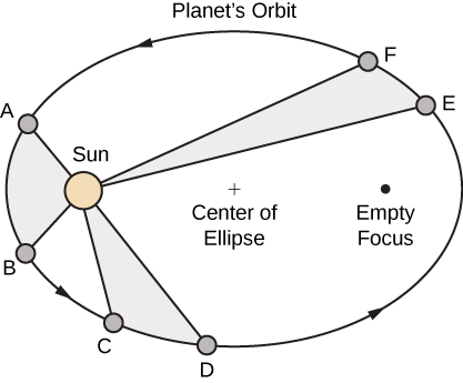
Figure 4. Kepler’s first and second laws are pictured here. The Sun is located at a focus of the elliptical orbit of any planet. Furthermore, the shaded areas are all equal, assuming that the amount of time measured as the planet moves is the same for each region.
Kepler’s third law is especially useful when using appropriate units. In particular, [latex]1\text{ }\textit{astronomical unit}[/latex] is defined to be the average distance from Earth to the Sun, and is now recognized to be [latex]149,597,870,700\text{ }m[/latex] or, approximately [latex]93,000,000[/latex]mi. We therefore write [latex]1\text{ }A.U. = 93,000,000[/latex]mi. Since the time it takes for Earth to orbit the Sun is [latex]1[/latex] year, we use Earth years for units of time. Then, substituting [latex]1[/latex] year for the period of Earth and [latex]1[/latex]A.U. for the average distance to the Sun, Kepler’s third law can be written as
[latex]T^2_p=D^3_p[/latex]
for any planet in the solar system, where [latex]T_p[/latex] is the period of that planet measured in Earth years and [latex]D_p[/latex] is the average distance from that planet to the Sun measured in astronomical units. Therefore, if we know the average distance from a planet to the Sun (in astronomical units), we can then calculate the length of its year (in Earth years), and vice versa.
Kepler’s laws were formulated based on observations from Brahe; however, they were not proved formally until Sir Isaac Newton was able to apply calculus. Furthermore, Newton was able to generalize Kepler’s third law to other orbital systems, such as a moon orbiting around a planet. Kepler’s original third law only applies to objects orbiting the Sun.
Proof
Let’s now prove Kepler’s first law using the calculus of vector-valued functions. First we need a coordinate system. Let’s place the Sun at the origin of the coordinate system and let the vector-valued function [latex]{\bf{r}}\,(t)[/latex] represent the location of a planet as a function of time. Newton proved Kepler’s law using his second law of motion and his law of universal gravitation. Newton’s second law of motion can be written as [latex]{\bf{F}}=m{\bf{a}}[/latex], where [latex]{\bf{F}}[/latex] represents the net force acting on the planet. His law of universal gravitation can be written in the form [latex]{\bf{F}}=-\frac{GmM}{\left\Vert{\bf{r}}\right\Vert^{2}}\cdot\frac{{\bf{r}}}{\left\Vert{\bf{r}}\right\Vert}[/latex], which indicates that the force resulting from the gravitational attraction of the Sun points back toward the Sun, and has magnitude [latex]\frac{GmM}{\left\Vert{\bf{r}}\right\Vert^{2}}[/latex] (Figure 9).
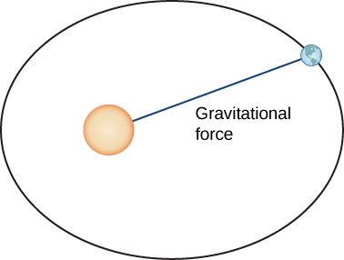
Figure 5. The gravitational force between Earth and the Sun is equal to the mass of the earth times its acceleration.
Setting these two forces equal to each other, and using the fact that [latex]{\bf{a}}\,(t)={\bf{v}}'\,(t)[/latex], we obtain
[latex]\large{m{\bf{v}}'\,(t)=-\frac{GmM}{\left\Vert{\bf{r}}\right\Vert^{2}}\cdot\frac{{\bf{r}}}{\left\Vert{\bf{r}}\right\Vert}}[/latex],
which can be rewritten as
[latex]\large{\frac{d{\bf{v}}}{dt}=-\frac{GM}{\left\Vert{\bf{r}}\right\Vert^{3}}{\bf{r}}}.[/latex]
This equation shows that the vectors [latex]d{\bf{v}}/dt[/latex] and [latex]{\bf{r}}[/latex] are parallel to each other, so [latex]d{\bf{v}}/dt\,\times\,{\bf{r}}=0[/latex]. Next, let’s differentiate [latex]{\bf{r}}\,\times\,{\bf{v}}[/latex] with respect to time:
[latex]\large{\frac{d}{dt}({\bf{r}}\,\times\,{\bf{v}})=\frac{d{\bf{r}}}{dt}\,\times\,{\bf{v}}+{\bf{r}}\,\times\frac{d{\bf{v}}}{dt}={\bf{v}}\,\times\,{\bf{v}}+{\bf{0}}={\bf{0}}}.[/latex]
This proves that [latex]{\bf{r}}\,\times\,{\bf{v}}[/latex] is a constant vector, which we call [latex]{\bf{C}}[/latex]. Since [latex]{\bf{r}}[/latex] and [latex]{\bf{v}}[/latex] are both perpendicular to [latex]{\bf{C}}[/latex] for all values of [latex]t[/latex], they must lie in a plane perpendicular to [latex]{\bf{C}}[/latex]. Therefore, the motion of the planet lies in a plane.
Next we calculate the expression [latex]d{\bf{v}}/dt\,\times\,{\bf{C}}[/latex]:
[latex]\frac{d{\bf{v}}}{dt}\,\times\,{\bf{C}}=-\frac{GM}{\left\Vert{\bf{r}}\right\Vert^{3}}{\bf{r}}\,\times\,({\bf{r}}\,\times\,{\bf{v}})=-\frac{GM}{\left\Vert{\bf{r}}\right\Vert^{3}}[({\bf{r}}\cdot{\bf{v}})\,{\bf{r}}-({\bf{r}}\cdot{\bf{r}})\,{\bf{v}}].[/latex]
The last equality in the above equation is from the triple cross product formula (Introduction to Vectors in Space). We need an expression for [latex]{\bf{r}}\cdot{\bf{v}}[/latex]. To calculate this, we differentiate [latex]{\bf{r}}\cdot{\bf{r}}[/latex] with respect to time:
[latex]\frac{d}{dt}({\bf{r}}\,\cdot\,{\bf{r}})=\frac{d{\bf{r}}}{dt}\cdot{\bf{r}}+{\bf{r}}\cdot\frac{d{\bf{r}}}{dt}=2{\bf{r}}\cdot\frac{d{\bf{r}}}{dt}=2{\bf{r}}\cdot{\bf{v}}.[/latex]
Since [latex]{\bf{r}}\,\cdot\,{\bf{r}}=\left\Vert{\bf{r}}\right\Vert^{2}[/latex], we also have
[latex]\frac{d}{dt}({\bf{r}}\cdot{\bf{r}})=\frac{d}{dt}\left\Vert{\bf{r}}\right\Vert^{2}=2\left\Vert{\bf{r}}\right\Vert\,\frac{d}{dt}\left\Vert{\bf{r}}\right\Vert[/latex].
Combining the last two equations, we get
[latex]\begin{array}{ccc}\hfill {2{\bf{r}}\cdot{\bf{v}}} & =\hfill & {2\left\Vert{\bf{r}}\right\Vert\,\frac{d}{dt}\left\Vert{\bf{r}}\right\Vert} \hfill \\ \hfill {{\bf{r}}\cdot{\bf{v}}}& =\hfill & {\left\Vert{\bf{r}}\right\Vert\,\frac{d}{dt}\left\Vert{\bf{r}}\right\Vert{.}}\hfill \\ \hfill \end{array}[/latex]
Substituting into our expression for [latex]\frac{d{\bf{v}}}{dt}\,\times\,{\bf{C}}[/latex] gives us
[latex]\begin{array}{ccc}\hfill {\frac{d{\bf{v}}}{dt}\,\times\,{\bf{C}}} & =\hfill & {-\frac{GM}{\left\Vert{\bf{r}}\right\Vert^{3}}[({\bf{r}}\cdot{\bf{r}})\,{\bf{r}}-({\bf{r}}\cdot{\bf{r}})\,{\bf{v}}]} \hfill \\ \hfill & =\hfill & {-\frac{GM}{\left\Vert{\bf{r}}\right\Vert^{3}}\big[\left\Vert{\bf{r}}\right\Vert{\big(}\frac{d}{dt}\left\Vert{\bf{r}}\right\Vert\big)\,{\bf{r}}-\left\Vert{\bf{r}}\right\Vert^{2}{\bf{v}}\big]}\hfill \\ \hfill & =\hfill & {-GM\Big[\frac{1}{\left\Vert{\bf{r}}\right\Vert^{2}}\big(\frac{d}{dt}\left\Vert{\bf{r}}\right\Vert\big)\,{\bf{r}}-\frac{1}{\left\Vert{\bf{r}}\right\Vert}{\bf{v}}\Big]}\hfill \\ \hfill & =\hfill & {GM\Big[\frac{\bf{v}}{\left\Vert{\bf{r}}\right\Vert}-\frac{{\bf{r}}}{\left\Vert{\bf{r}}\right\Vert^{2}}\big(\frac{d}{dt}\left\Vert{\bf{r}}\right\Vert\big)\Big].}\hfill \\ \hfill \end{array}[/latex]
However,
[latex]\begin{array}{ccc}\hfill {\frac{d}{dt}\,\frac{{\bf{r}}}{\left\Vert{\bf{r}}\right\Vert}} & =\hfill & {\frac{\frac{d}{dt}({\bf{r}})\left\Vert{\bf{r}}\right\Vert-{\bf{r}}\frac{d}{dt}\left\Vert{\bf{r}}\right\Vert}{\left\Vert{\bf{r}}\right\Vert}} \hfill \\ \hfill & =\hfill & {\frac{\frac{d{\bf{r}}}{dt}}{\left\Vert{\bf{r}}\right\Vert}-\frac{{\bf{r}}}{\left\Vert{\bf{r}}\right\Vert^{2}}\,\frac{d}{dt}\left\Vert{\bf{r}}\right\Vert}\hfill \\ \hfill & =\hfill & {\frac{\bf{v}}{\left\Vert{\bf{r}}\right\Vert}-\frac{{\bf{r}}}{\left\Vert{\bf{v}}\right\Vert^{2}}\,\frac{d}{dt}\left\Vert{\bf{r}}\right\Vert.}\hfill \\ \hfill \end{array}[/latex]
Therefore, we get
[latex]\large{\frac{d{\bf{v}}}{dt}\,\times\,{\bf{C}}=GM\Big(\frac{d}{dt}\,\frac{\bf{r}}{\left\Vert{\bf{r}}\right\Vert}\Big)}.[/latex]
Since [latex]\bf{C}[/latex] is a constant vector, we can integrate both sides and obtain
[latex]{\bf{v}}\,\times\,{\bf{C}}=GM\frac{{\bf{r}}}{\left\Vert{\bf{r}}\right\Vert}+{\bf{D}},[/latex]
where [latex]\bf{D}[/latex] is a constant vector. Our goal is to solve for [latex]\left\Vert{\bf{r}}\right\Vert[/latex]. Let’s start by calculating [latex]{\bf{r}}\cdot({\bf{v}}\,\times\,{\bf{C}})[/latex]:
[latex]{\bf{r}}\cdot({\bf{v}}\,\times\,{\bf{C}})={\bf{r}}\cdot\Big(GM\frac{\bf{r}}{\left\Vert{\bf{r}}\right\Vert}+{\bf{D}}\Big)=GM\frac{\left\Vert{\bf{r}}\right\Vert^{2}}{\left\Vert{\bf{r}}\right\Vert}+{\bf{r}}\cdot{\bf{D}}=GM\left\Vert{\bf{r}}\right\Vert+{\bf{r}}\cdot{\bf{D}}.[/latex]
However, [latex]{\bf{r}}\cdot({\bf{v}}\,\times\,{\bf{C}})=({\bf{r}}\,\times\,{\bf{v}})\,\times\,{\bf{C}}[/latex], so
[latex]({\bf{r}}\,\times\,{\bf{v}})\,\times\,{\bf{C}}=GM\left\Vert{\bf{r}}\right\Vert+{\bf{r}}\cdot{\bf{D}}[/latex].
Since [latex]{\bf{r}}\,\times\,{\bf{v}}={\bf{C}}[/latex], we have
[latex]\left\Vert{\bf{C}}\right\Vert^{2}=GM\left\Vert{\bf{r}}\right\Vert+{\bf{r}}\cdot{\bf{D}}[/latex].
Note that [latex]{\bf{r}}\cdot{\bf{D}}=\left\Vert{\bf{r}}\right\Vert\,\left\Vert{\bf{D}}\right\Vert\cos{\theta}[/latex], where [latex]\theta[/latex] is the angle between [latex]\bf{r}[/latex] and [latex]\bf{D}[/latex]. Therefore,
[latex]\left\Vert{\bf{C}}\right\Vert^{2}=GM\left\Vert{\bf{r}}\right\Vert+\left\Vert{\bf{r}}\right\Vert\,\left\Vert{\bf{D}}\right\Vert\cos{\theta}[/latex].
Solving for [latex]\left\Vert{\bf{r}}\right\Vert[/latex],
[latex]\left\Vert{\bf{r}}\right\Vert=\frac{\left\Vert{\bf{C}}\right\Vert^{2}}{GM+\left\Vert{\bf{D}}\right\Vert\cos{\theta}}=\frac{\left\Vert{\bf{C}}\right\Vert^{2}}{GM}\bigg(\frac{1}{1+e\cos{\theta}}\bigg)[/latex],
where [latex]e=\left\Vert{\bf{D}}\right\Vert/GM[/latex]. This is the polar equation of a conic with a focus at the origin, which we set up to be the Sun. It is a hyperbola if [latex]e\,>\,1[/latex], a parabola if [latex]e=1[/latex], or an ellipse if [latex]e\,<\,1[/latex]. Since planets have closed orbits, the only possibility is an ellipse. However, at this point it should be mentioned that hyperbolic comets do exist. These are objects that are merely passing through the solar system at speeds too great to be trapped into orbit around the Sun. As they pass close enough to the Sun, the gravitational field of the Sun deflects the trajectory enough so the path becomes hyperbolic. [latex]_\blacksquare[/latex]
Example: Using Kepler’s Third Law for Nonheliocentric Orbits
Kepler’s third law of planetary motion can be modified to the case of one object in orbit around an object other than the Sun, such as the Moon around the Earth. In this case, Kepler’s third law becomes
[latex]\large{P^{2}=\frac{4\pi^{2}a^{3}}{G(m+M)}},[/latex]
where [latex]m[/latex] is the mass of the Moon and [latex]M[/latex] is the mass of Earth, [latex]a[/latex] represents the length of the major axis of the elliptical orbit, and [latex]P[/latex] represents the period.
Given that the mass of the Moon is [latex]7.35\ \times\ 10^{22}\text{ kg}[/latex], the mass of the Earth is [latex]5.97\ \times\ 10^{24}\text{ kg}[/latex],
[latex]G=6.67\ \times\ 10^{-11}\text{m}_{\small{3}}/\text{kg}\cdot\text{sec}^{2}[/latex], and the period of the moon is [latex]27.3[/latex] days, let’s find the length of the major axis of the orbit of the Moon around Earth.
Analysis
According to solarsystem.nasa.gov, the actual average distance from the Moon to Earth is [latex]384,400\text{ km}[/latex]. This is calculated using reflectors left on the Moon by Apollo astronauts back in the 1960s.
try it
Titan is the largest moon of Saturn. The mass of Titan is approximately [latex]1.35\,\times\,10^{23}\text{ kg}[/latex]. The mass of Saturn is approximately [latex]5.68\,\times\,10^{26}\text{ kg}[/latex]. Titan takes approximately [latex]16[/latex] days to orbit Saturn. Use this information, along with the universal gravitation constant [latex]G=6.67\,\times\,10^{-11}\text{ m}^{3}/\text{kg}\cdot{\text{sec}}^{2}[/latex] to estimate the distance from Titan to Saturn.
Watch the following video to see the worked solution to the above Try It
Activity: Navigating a Banked Turn
How fast can a racecar travel through a circular turn without skidding and hitting the wall? The answer could depend on several factors:
- The weight of the car;
- The friction between the tires and the road;
- The radius of the circle;
- The “steepness” of the turn;
In this project we investigate this question for NASCAR racecars at the Bristol Motor Speedway in Tennessee. Before considering this track in particular, we use vector functions to develop the mathematics and physics necessary for answering questions such as this.
A car of mass [latex]m[/latex] moves with constant angular speed [latex]\omega[/latex] around a circular curve of radius [latex]R[/latex] (Figure 10). The curve is banked at an angle [latex]\theta[/latex]. If the height of the car off the ground is [latex]h[/latex], then the position of the car at time [latex]t[/latex] is given by the function [latex]r(t)=\langle{\bf{R}}\cos{(\omega{t})},\ {\bf{R}}\sin{(\omega{t})},\ h\rangle[/latex].
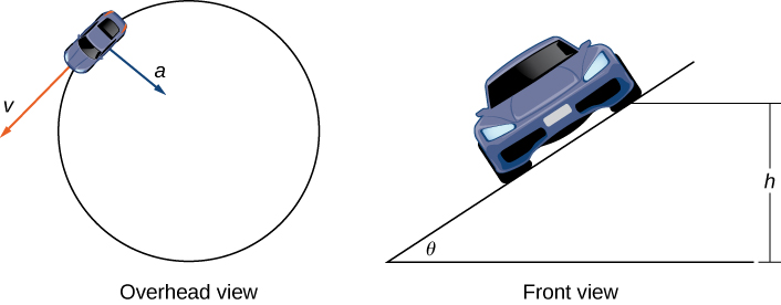
Figure 6. Views of a race car moving around a track.
- Find the velocity function [latex]{\bf{v}}\,(t)[/latex] of the car. Show that [latex]{\bf{v}}[/latex] is tangent to the circular curve. This means that, without a force to keep the car on the curve, the car will shoot off of it.
- Show that the speed of the car is [latex]\omega{R}[/latex]. Use this to show that [latex](2\pi{r})\,/\,{\bf{v}}=(2\pi)\,/\,\omega[/latex].
- Find the acceleration [latex]{\bf{a}}[/latex]. Show that this vector points toward the center of the circle and that [latex]|{\bf{a}}|=R\omega^{2}[/latex].
- The force required to produce this circular motion is called the centripetal force, and it is denoted [latex]{\bf{F}}_{\text{cent}}[/latex]. This force points toward the center of the circle (not toward the ground). Show that [latex]|{\bf{F}}_{\text{cent}}|=(m|{\bf{v}}|^{2})\,/\,R[/latex]. As the car moves around the curve, three forces act on it: gravity, the force exerted by the road (this force is perpendicular to the ground), and the friction force (Figure 11). Because describing the frictional force generated by the tires and the road is complex, we use a standard approximation for the frictional force. Assume that [latex]|{\bf{f}}|=\mu|{\bf{N}}|[/latex]for some positive constant [latex]\mu[/latex]. The constant [latex]\mu[/latex] is called the coefficient of friction.

Figure 7. The car has three forces acting on it: gravity (denoted by [latex]m{\bf{g}}[/latex]), the friction force [latex]\bf{f}[/latex], and the force exerted by the road [latex]\bf{N}[/latex].
Let [latex]v_{\text{max}}[/latex] denote the maximum speed the car can attain through the curve without skidding. In other words, [latex]v_{\text{max}}[/latex] is the fastest speed at which the car can navigate the turn. When the car is traveling at this speed, the magnitude of the centripetal force is
[latex]|\large{{\bf{F}}_{\text{cent}}|=\frac{mv^{2}_{\text{max}}}{R}}[/latex].The next three questions deal with developing a formula that relates the speed [latex]v_{\text{max}}[/latex] to the banking angle [latex]\theta[/latex].
- Show that [latex]|{\bf{N}}|\cos{\theta}=mg+|{\bf{f}}|\sin{\theta}[/latex]. Conclude that [latex]|{bf{N}}|=(mg)\,/\,(\cos{\theta}-\mu\sin{\theta})[/latex].
- The centripetal force is the sum of the forces in the horizontal direction, since the centripetal force points toward the center of the circular curve. Show that
[latex]|{\bf{F}}_{\text{cent}}|=|{\bf{N}}|\sin{\theta}+|{\bf{f}}|\cos{\theta}[/latex].
Conclude that
[latex]|\large{{\bf{F}}_{\text{cent}}|=\frac{\sin{\theta}+\mu\cos{\theta}}{\cos{\theta}-\mu\sin{\theta}}mg}[/latex]. - Show that [latex]\text{v}^{2}_{\text{max}}=((\sin{\theta}+\mu\cos{\theta}) \ / \ (\cos{\theta}-\mu\sin{\theta}))gR[/latex]. Conclude that the maximum speed does not actually depend on the mass of the car.
Now that we have a formula relating the maximum speed of the car and the banking angle, we are in a position to answer the questions like the one posed at the beginning of the project.
The Bristol Motor Speedway is a NASCAR short track in Bristol, Tennessee. The track has the approximate shape shown in Figure 12. Each end of the track is approximately semicircular, so when cars make turns they are traveling along an approximately circular curve. If a car takes the inside track and speeds along the bottom of turn 1, the car travels along a semicircle of radius approximately [latex]211\ ft[/latex] with a banking angle of [latex]24^{\circ}[/latex]. If the car decides to take the outside track and speeds along the top of turn 1, then the car travels along a semicircle with a banking angle of [latex]28^{\circ}[/latex]. (The track has variable angle banking.)
Figure 8. At the Bristol Motor Speedway, Bristol, Tennessee (a), the turns have an inner radius of about 211 ft and a width of 40 ft (b). (credit: part (a) photo by Raniel Diaz, Flickr)
The coefficient of friction for a normal tire in dry conditions is approximately [latex]0.7[/latex]. Therefore, we assume the coefficient for a NASCAR tire in dry conditions is approximately [latex]0.98[/latex].
Before answering the following questions, note that it is easier to do computations in terms of feet and seconds, and then convert the answers to miles per hour as a final step.
- In dry conditions, how fast can the car travel through the bottom of the turn without skidding?
- In dry conditions, how fast can the car travel through the top of the turn without skidding?
- In wet conditions, the coefficient of friction can become as low as [latex]0.1[/latex]. If this is the case, how fast can the car travel through the bottom of the turn without skidding?
- Suppose the measured speed of a car going along the outside edge of the turn is [latex]105\text{ mph}[/latex]. Estimate the coefficient of friction for the car’s tires.
Candela Citations
- CP 3.16. Authored by: Ryan Melton. License: CC BY: Attribution
- CP 3.17. Authored by: Ryan Melton. License: CC BY: Attribution
- Calculus Volume 3. Authored by: Gilbert Strang, Edwin (Jed) Herman. Provided by: OpenStax. Located at: https://openstax.org/books/calculus-volume-3/pages/1-introduction. License: CC BY-NC-SA: Attribution-NonCommercial-ShareAlike. License Terms: Access for free at https://openstax.org/books/calculus-volume-3/pages/1-introduction
