Profitable Golf Balls

Figure 1.

Pro-$T$ company has developed a profit model that depends on the number $x$ of golf balls sold per month (measured in thousands), and the number of hours per month of advertising $y$, according to the function

$z=f(x,y)=48x+96y-x^{2}-2xy-9y^{2}$

where $z$ is measured in thousands of dollars. The maximum number of golf balls that can be produced and sold is $50,000$, and the maximum number of hours of advertising that can be purchased is $25$. Find the values of $x$ and $y$ that maximize profit, and find the maximum profit.

Solution

Using the problem-solving strategy, step 1 involves finding the critical points of $f$ on its domain. Therefore, we first calculate $f_{x}(x,y)$ and $f_{y}(x,y)$, then set them each equal to zero:

$\begin{array}{c}f_{x}(x,y) &=& 48-2x-2y \hfill \\f_{y}(x,y) &=& 96-2x-18y \hfill \end{array}$

Setting them equal to zero yields the system of equations

$\begin{array}{c}48-2x-2y &=& 0 \hfill \\96-2x-18y &=& 0 \hfill \end{array}$

The solution to this system is $x=21$ and $y=3$. Therefore $(21,3)$ is a critical point of $f$. Calculating $f(21,3)$ gives $f(21,3)=48(21)+96(3)-21^{2}-2(21)(3)-9(3)^{2}=648$.

The domain of this function is $0\le{x}\le{50}$ and $0\le{y}\le{25}$ as shown in the following graph.

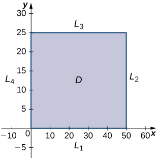
Figure 2. Graph of the domain of the function$z=f(x,y)=48x+96y-x^{2}-2xy-9y^{2}$.

$L_{1}$ is the line segment connecting $(0,0)$ and $(50,0)$, and it can be parameterized by the equations $x(t)=t$, $y(t)=0$ for $0\le{t}\le{50}$. We then define $g(t)=f(x(t),y(t))$:

$\begin{array}{c}g(t) &=&f(x(t),y(t)) \hfill \\ &=& f(t,0) \hfill \\ &=& 48t+96(0)-y^{2}-2(t)(0)-9(0)^{2} \hfill \\ &=& 48t-t^{2} \hfill \end{array}$

Setting $g^{\prime}(t)=0$ yields the critical point $t=24$, which corresponds to the point $(24,0)$ in the domain of $f$. Calculating $f(24,0)$ gives $576$.

$L_{2}$ is the line segment connecting $(50,0)$ and $(50,25)$, and it can be parameterized by the equations $x(t)=50$, $y(t)=t$ for $0\le{t}\le{25}$. Once again we define $g(t)=f(x(t),y(t))$:

$\begin{array}{c}g(t) &=&f(x(t),y(t)) \hfill \\ &=& f(50,t) \hfill \\ &=& 48(50)+96t-50^{2}-2(50)t-9t^{2} \hfill \\ &=& -9t^{2}-4t-100 \hfill \end{array}$

This function has a critical point $t=-\frac{2}{9}$, which corresponds to the point $(50,-\frac{2}{9})$. This point is not in the domain of $f$.

$L_{3}$ is the line segment connecting $(0,25)$ and $(50,25)$, and it can be parameterized by the equations $x(t)=t$, $y(t)=25$ for $0\le{t}\le{50}$. We define $g(t)=f(x(t),y(t))$:

$\begin{array}{c}g(t) &=&f(x(t),y(t)) \hfill \\ &=& f(t,25) \hfill \\ &=& 48(t)+96(25)-t^{2}-2t(25)-9(25)^{2} \hfill \\ &=& -t^{2}-2t-3225 \hfill \end{array}$

This function has a critical point $t=-1$, which corresponds to the point $(-1,25)$, which is not in the domain.

$L_{4}$ is the line segment connecting $(0)$ and $(0,25)$, and it can be parameterized by the equations $x(t)=0$, $y(t)=t$ for $0\le{t}\le{25}$. We define $g(t)=f(x(t),y(t))$:

$\begin{array}{c}g(t) &=&f(x(t),y(t)) \hfill \\ &=& f(0,t) \hfill \\ &=& 48(0)+96t-(0)^{2}-2(0)t-9t^{2} \hfill \\ &=& 96t-t^{2} \hfill \end{array}$

This function has a critical point $t=\frac{16}{3}$, which corresponds to the point $(0,\frac{16}{3})$, which is on the boundary of the domain. Calculating $f(0,\frac{16}{3})$ gives $256$.

We also need to find the values of $f(x,y)$ at the corners of its domain. These corners are located at $(0,0),(50,0),(50,25),\text{ and }(0,25)$:

$\begin{array}{c}f(0,0) &=& 48(0)+96(0)-(0)^{2}-2(0)(0)-9(0)^{2}=0 \hfill \\f(50,0) &=& 48(50)+96(0)-(50)^{2}-2(50)(0)-9(0)^{2}=-100 \hfill \\f(50,25) &=& 48(50)+96(25)-(500)^{2}-2(50)(25)-9(25)^{2}=-5825 \hfill \\f(0,25) &=& 48(0)+96(25)-(0)^{2}-2(0)(25)-9(25)^{2}=-3225 \hfill \end{array}$

The maximum critical value is $648$ which occurs at $(21,3)$. Therefore, a maximum profit of $\$648,000$ is realized when $21,000$ golf balls are sold and $33$ hours of advertising are purchased per month as shown in the following figure.

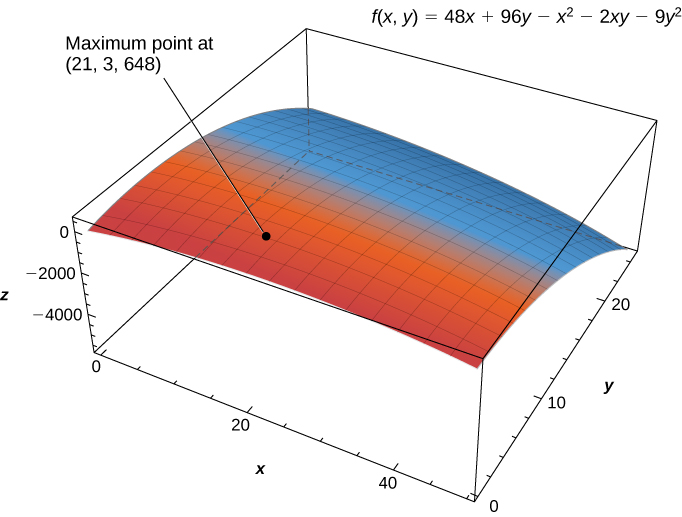
Figure 3. The profit function $f(x,y)$ has a maximum at $(21,3,648)$.