Learning Objectives
- Explain the meaning of an oriented surface, giving an example.
- Describe the surface integral of a vector field.
- Use surface integrals to solve applied problems.
Orientation of a Surface
Recall that when we defined a scalar line integral, we did not need to worry about an orientation of the curve of integration. The same was true for scalar surface integrals: we did not need to worry about an “orientation” of the surface of integration.
On the other hand, when we defined vector line integrals, the curve of integration needed an orientation. That is, we needed the notion of an oriented curve to define a vector line integral without ambiguity. Similarly, when we define a surface integral of a vector field, we need the notion of an oriented surface. An oriented surface is given an “upward” or “downward” orientation or, in the case of surfaces such as a sphere or cylinder, an “outward” or “inward” orientation.
Let [latex]S[/latex] be a smooth surface. For any point [latex](x, y, z)[/latex] on [latex]S[/latex], we can identify two unit normal vectors [latex]N[/latex] and [latex]-N[/latex]. If it is possible to choose a unit normal vector [latex]{\bf{N}}[/latex] at every point [latex](x, y, z)[/latex] on [latex]S[/latex] so that [latex]{\bf{N}}[/latex] varies continuously over [latex]S[/latex], then [latex]S[/latex] is “orientable.” Such a choice of unit normal vector at each point gives the orientation of a surface [latex]S[/latex]. If you think of the normal field as describing water flow, then the side of the surface that water flows toward is the “negative” side and the side of the surface at which the water flows away is the “positive” side. Informally, a choice of orientation gives [latex]S[/latex] an “outer” side and an “inner” side (or an “upward” side and a “downward” side), just as a choice of orientation of a curve gives the curve “forward” and “backward” directions.
Closed surfaces such as spheres are orientable: if we choose the outward normal vector at each point on the surface of the sphere, then the unit normal vectors vary continuously. This is called the positive orientation of the closed surface (Figure 1). We also could choose the inward normal vector at each point to give an “inward” orientation, which is the negative orientation of the surface.

Figure 1. An oriented sphere with positive orientation.
A portion of the graph of any smooth function [latex]z=f(x, y)[/latex] is also orientable. If we choose the unit normal vector that points “above” the surface at each point, then the unit normal vectors vary continuously over the surface. We could also choose the unit normal vector that points “below” the surface at each point. To get such an orientation, we parameterize the graph of [latex]f[/latex] in the standard way: [latex]{\bf{r}}(x,y)=\langle{x},y,f(x,y)\rangle[/latex], where [latex]x[/latex] and [latex]y[/latex] vary over the domain of [latex]f[/latex]. Then, [latex]{\bf{t}}_x=\langle1,0,f_x\rangle[/latex] and [latex]{\bf{t}}_y=\langle0,1,f_y\rangle[/latex], and therefore the cross product [latex]{\bf{t}}_x\times{\bf{t}}_y[/latex] (which is normal to the surface at any point on the surface) is [latex]\langle-f_x,-f_y,1\rangle[/latex]. Since the [latex]z[/latex] component of this vector is one, the corresponding unit normal vector points “upward,” and the upward side of the surface is chosen to be the “positive” side.
Let [latex]S[/latex] be a smooth orientable surface with parameterization [latex]{\bf{r}}(u,v)[/latex]. For each point [latex]{\bf{r}}(a,b)[/latex] on the surface, vectors [latex]{\bf{t}}_u[/latex] and [latex]{\bf{t}}_v[/latex] lie in the tangent plane at that point. Vector [latex]{\bf{t}}_u\times{\bf{t}}_v[/latex] is normal to the tangent plane at [latex]{\bf{r}}(a,b)[/latex] and is therefore normal to [latex]S[/latex] at that point. Therefore, the choice of unit normal vector
[latex]\large{{\bf{N}}=\frac{{\bf{t}}_u\times{\bf{t}}_v}{||{\bf{t}}_u\times{\bf{t}}_v||}}[/latex]
gives an orientation of surface [latex]S[/latex].
Example: choosing an orientation
Give an orientation of cylinder [latex]x^2+y^2=r^2[/latex], [latex]0\leq{z}\leq{h}[/latex].

try it
Give the “upward” orientation of the graph of [latex]f(x, y)=xy[/latex].
Since every curve has a “forward” and “backward” direction (or, in the case of a closed curve, a clockwise and counterclockwise direction), it is possible to give an orientation to any curve. Hence, it is possible to think of every curve as an oriented curve. This is not the case with surfaces, however. Some surfaces cannot be oriented; such surfaces are called nonorientable. Essentially, a surface can be oriented if the surface has an “inner” side and an “outer” side, or an “upward” side and a “downward” side. Some surfaces are twisted in such a fashion that there is no well-defined notion of an “inner” or “outer” side.
The classic example of a nonorientable surface is the Möbius strip. To create a Möbius strip, take a rectangular strip of paper, give the piece of paper a half-twist, and the glue the ends together (Figure 3). Because of the half-twist in the strip, the surface has no “outer” side or “inner” side. If you imagine placing a normal vector at a point on the strip and having the vector travel all the way around the band, then (because of the half-twist) the vector points in the opposite direction when it gets back to its original position. Therefore, the strip really only has one side.

Figure 3. The construction of a Möbius strip.
Since some surfaces are nonorientable, it is not possible to define a vector surface integral on all piecewise smooth surfaces. This is in contrast to vector line integrals, which can be defined on any piecewise smooth curve.
Surface Integral of a Vector Field
With the idea of orientable surfaces in place, we are now ready to define a surface integral of a vector field. The definition is analogous to the definition of the flux of a vector field along a plane curve. Recall that if [latex]{\bf{F}}[/latex] is a two-dimensional vector field and [latex]C[/latex] is a plane curve, then the definition of the flux of [latex]{\bf{F}}[/latex] along [latex]C[/latex] involved chopping [latex]C[/latex] into small pieces, choosing a point inside each piece, and calculating [latex]{\bf{F}}\cdot{\bf{N}}[/latex] at the point (where [latex]{\bf{N}}[/latex] is the unit normal vector at the point). The definition of a surface integral of a vector field proceeds in the same fashion, except now we chop surface [latex]S[/latex] into small pieces, choose a point in the small (two-dimensional) piece, and calculate [latex]{\bf{F}}\cdot{\bf{N}}[/latex] at the point.
To place this definition in a real-world setting, let [latex]S[/latex] be an oriented surface with unit normal vector [latex]{\bf{N}}[/latex]. Let [latex]{\bf{v}}[/latex] be a velocity field of a fluid flowing through [latex]S[/latex], and suppose the fluid has density [latex]\rho(x,y,z)[/latex]. Imagine the fluid flows through [latex]S[/latex], but [latex]S[/latex] is completely permeable so that it does not impede the fluid flow (Figure 4). The mass flux of the fluid is the rate of mass flow per unit area. The mass flux is measured in mass per unit time per unit area. How could we calculate the mass flux of the fluid across [latex]S[/latex]?

Figure 4. Fluid flows across a completely permeable surface [latex]S[/latex].
The rate of flow, measured in mass per unit time per unit area, is [latex]\rho{\bf{N}}[/latex]. To calculate the mass flux across [latex]S[/latex], chop [latex]S[/latex] into small pieces [latex]S_{ij}[/latex]. If [latex]S_{ij}[/latex] is small enough, then it can be approximated by a tangent plane at some point [latex]P[/latex] in [latex]S_{ij}[/latex]. Therefore, the unit normal vector at [latex]P[/latex] can be used to approximate [latex]{\bf{N}}(x,y,z)[/latex] across the entire piece [latex]S_{ij}[/latex], because the normal vector to a plane does not change as we move across the plane. The component of the vector [latex]\rho{\bf{v}}[/latex] at [latex]P[/latex] in the direction of [latex]{\bf{N}}[/latex] is [latex]\rho{\bf{v}}\cdot{\bf{N}}[/latex] at [latex]P[/latex]. Since [latex]S_{ij}[/latex] is small, the dot product [latex]\rho{\bf{v}}\cdot{\bf{N}}[/latex] changes very little as we vary across [latex]S_{ij}[/latex], and therefore [latex]\rho{\bf{v}}\cdot{\bf{N}}[/latex] can be taken as approximately constant across [latex]S_{ij}[/latex]. To approximate the mass of fluid per unit time flowing across [latex]S_{ij}[/latex] (and not just locally at point [latex]P[/latex]), we need to multiply [latex](\rho{\bf{v}}\cdot{\bf{N}})(P)[/latex] by the area of [latex]S_{ij}[/latex]. Therefore, the mass of fluid per unit time flowing across [latex]S_{ij}[/latex] in the direction of [latex]{\bf{N}}[/latex] can be approximated by [latex](\rho{\bf{v}}\cdot{\bf{N}})\nabla{S_{ij}}[/latex], where [latex]{\bf{N}}[/latex], [latex]\rho[/latex], and [latex]{\bf{v}}[/latex] are all evaluated at [latex]P[/latex] (Figure 5). This is analogous to the flux of two-dimensional vector field [latex]{\bf{F}}[/latex] across plane curve [latex]C[/latex], in which we approximated flux across a small piece of [latex]C[/latex] with the expression [latex]({\bf{F}}\cdot{\bf{N}})\nabla{s}[/latex]. To approximate the mass flux across [latex]S[/latex], form the sum [latex]\displaystyle\sum_{i=1}^m\displaystyle\sum_{j=1}^n(\rho{\bf{v}}\cdot{\bf{N}})\nabla{S_{ij}}[/latex]. As pieces [latex]S_{ij}[/latex] get smaller, the sum [latex]\displaystyle\sum_{i=1}^m\displaystyle\sum_{j=1}^n(\rho{\bf{v}}\cdot{\bf{N}})\nabla{S_{ij}}[/latex] gets arbitrarily close to the mass flux. Therefore, the mass flux is
[latex]\displaystyle\iint_s\rho{\bf{v}}\cdot{\bf{N}}dS=\displaystyle\lim_{m,n\to\infty}\displaystyle\sum_{i=1}^m\displaystyle\sum_{j=1}^n(\rho{\bf{v}}\cdot{\bf{N}})\nabla{S_{ij}}[/latex].
This is a surface integral of a vector field. Letting the vector field [latex]\rho{\bf{v}}[/latex] be an arbitrary vector field [latex]{\bf{F}}[/latex] leads to the following definition.
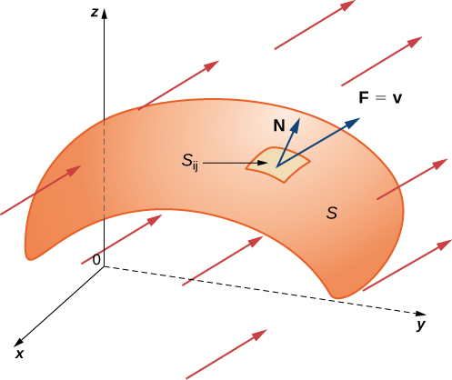
Figure 5. The mass of fluid per unit time flowing across [latex]S_{ij}[/latex] in the direction of [latex]{\bf{N}}[/latex] can be approximated by [latex](\rho{\bf{v}}\cdot{\bf{N}})\nabla{S_{ij}}[/latex].
Definition
Let [latex]{\bf{F}}[/latex] be a continuous vector field with a domain that contains oriented surface [latex]S[/latex] with unit normal vector [latex]{\bf{N}}[/latex]. The surface integral of [latex]{\bf{F}}[/latex] over [latex]S[/latex] is
[latex]\displaystyle\iint_S{\bf{F}}\cdot{d}S=\displaystyle\iint_S{\bf{F}}\cdot{\bf{N}}{d}S[/latex].
Notice the parallel between this definition and the definition of vector line integral [latex]\displaystyle\int_C{\bf{F}}\cdot{\bf{N}}{d}s[/latex]. A surface integral of a vector field is defined in a similar way to a flux line integral across a curve, except the domain of integration is a surface (a two-dimensional object) rather than a curve (a one-dimensional object). Integral [latex]\displaystyle\iint_S{\bf{F}}\cdot{\bf{N}}{d}S[/latex] is called the flux of [latex]{\bf{F}}[/latex] across [latex]S[/latex], just as integral [latex]\displaystyle\int_C{\bf{F}}\cdot{\bf{N}}{d}s[/latex] is the flux of [latex]{\bf{F}}[/latex] across curve [latex]C[/latex]. A surface integral over a vector field is also called a flux integral.
Just as with vector line integrals, surface integral [latex]\displaystyle\iint_S{\bf{F}}\cdot{\bf{N}}{d}S[/latex] is easier to compute after surface [latex]S[/latex] has been parameterized. Let [latex]{\bf{r}}(u,v)[/latex] be a parameterization of [latex]S[/latex] with parameter domain [latex]D[/latex]. Then, the unit normal vector is given by [latex]{\bf{N}}=\frac{{\bf{t}}_u\times{\bf{t}}_v}{||{\bf{t}}_u\times{\bf{t}}_v||}[/latex] and, from the surface integral equation, we have
[latex]\begin{aligned} \displaystyle\iint_S{\bf{F}}\cdot{\bf{N}}{d}S&=\displaystyle\iint_S{\bf{F}}\cdot{\bf{N}}{d}S \\ &=\displaystyle\iint_S{\bf{F}}\cdot\frac{{\bf{t}}_u\times{\bf{t}}_v}{||{\bf{t}}_u\times{\bf{t}}_v||}dS \\ &=\displaystyle\iint_D\left({\bf{F}}({\bf{r}}(u,v))\cdot\frac{{\bf{t}}_u\times{\bf{t}}_v}{||{\bf{t}}_u\times{\bf{t}}_v||}\right)||{\bf{t}}_u\times{\bf{t}}_v||dA \\ &=\displaystyle\iint_D({\bf{F}}({\bf{r}}(u,v))\cdot({\bf{t}}_u\times{\bf{t}}_v))dA \end{aligned}[/latex].
Therefore, to compute a surface integral over a vector field we can use the equation
[latex]\displaystyle\iint_S{\bf{F}}\cdot{\bf{N}}{d}S=\displaystyle\iint_D({\bf{F}}({\bf{r}}(u,v))\cdot({\bf{t}}_u\times{\bf{t}}_v))dA[/latex].
Example: calculating a surface integral
Calculate the surface integral [latex]\displaystyle\iint_S{\bf{F}}\cdot{\bf{N}}{d}S[/latex], where [latex]{\bf{F}}=\langle-y,x,0\rangle[/latex] and [latex]S[/latex] is the surface with parameterization [latex]{\bf{r}}(u,v)=\langle{u},v^2-u,u+v\rangle[/latex], [latex]0\leq{u}\leq3, \ 0\leq{v}\leq4[/latex].
try it
Calculate surface integral [latex]\displaystyle\iint_S{\bf{F}}\cdot{d}S[/latex], where [latex]{\bf{F}}=\langle0,-z,y\rangle[/latex] and [latex]S[/latex] is the portion of the unit sphere in the first octant with outward orientation.
Watch the following video to see the worked solution to the above Try It
Example: calculating mass flow rate
Let [latex]{\bf{v}}(x,y,z)=\langle2x,2y,z\rangle[/latex] represent a velocity field (with units of meters per second) of a fluid with constant density [latex]80[/latex] kg/m3. Let [latex]S[/latex] be hemisphere [latex]x^{2}+y^{2}+z^{2}=9[/latex] with [latex]z\geq 0[/latex] such that [latex]S[/latex] is oriented outward. Find the mass flow rate of the fluid across [latex]S[/latex].
try it
Let [latex]{\bf{v}}(x,y,z)=\langle{x}^2+y^2,z,4y\rangle[/latex] m/sec represent a velocity field of a fluid with constant density [latex]100[/latex] kg/m3. Let [latex]S[/latex] be the half-cylinder [latex]{\bf{r}}(u,v)=\langle\cos{u},\sin{u},v\rangle[/latex], [latex]0\leq{u}\leq\pi, \ 0\leq{v}\leq2[/latex] oriented outward. Calculate the mass flux of the fluid across [latex]S[/latex].
In Example “Calculating A Surface Integral”, we computed the mass flux, which is the rate of mass flow per unit area. If we want to find the flow rate (measured in volume per time) instead, we can use flux integral [latex]\displaystyle\int \ \displaystyle\int_S{\bf{v}}\cdot{\bf{N}}dS[/latex], which leaves out the density. Since the flow rate of a fluid is measured in volume per unit time, flow rate does not take mass into account. Therefore, we have the following characterization of the flow rate of a fluid with velocity [latex]{\bf{v}}[/latex] across a surface [latex]S[/latex]:
Flow rate of fluid across [latex]\displaystyle\int \ \displaystyle\int_S{\bf{v}}\cdot{\bf{N}}dS[/latex].
To compute the flow rate of the fluid in Example “Calculating the Mass of a Sheet”, we simply remove the density constant, which gives a flow rate of [latex]90\pi\text{ m^3/sec}[/latex].
Both mass flux and flow rate are important in physics and engineering. Mass flux measures how much mass is flowing across a surface; flow rate measures how much volume of fluid is flowing across a surface.
In addition to modeling fluid flow, surface integrals can be used to model heat flow. Suppose that the temperature at point [latex](x, y, z)[/latex] in an object is [latex]T(x, y, z)[/latex]. Then the heat flow is a vector field proportional to the negative temperature gradient in the object. To be precise, the heat flow is defined as vector field [latex]{\bf{F}}=-k\nabla{t}[/latex], where the constant [latex]k[/latex] is the thermal conductivity of the substance from which the object is made (this constant is determined experimentally). The rate of heat flow across surface [latex]S[/latex] in the object is given by the flux integral
[latex]\large{\displaystyle\iint_S{\bf{F}}\cdot{d}{\bf{S}}=\displaystyle\iint_S-k\nabla{T}\cdot{d}{\bf{S}}}[/latex].
Example: calculating heat flow
A cast-iron solid cylinder is given by inequalities [latex]x^2+y^2\leq1[/latex], [latex]1\leq{z}\leq4[/latex]. The temperature at point [latex](x, y, z)[/latex] in a region containing the cylinder is [latex]T(x,y,z)=(x^2+y^2)z[/latex]. Given that the thermal conductivity of cast iron is 55, find the heat flow across the boundary of the solid if this boundary is oriented outward.
try it
A cast-iron solid ball is given by inequality [latex]x^2+y^2+z^2\leq1[/latex]. The temperature at a point in a region containing the ball is [latex]T(x,y,z)=\frac13(x^2+y^2+z^2)[/latex]. Find the heat flow across the boundary of the solid if this boundary is oriented outward.
Candela Citations
- CP 6.58. Authored by: Ryan Melton. License: CC BY: Attribution
- Calculus Volume 3. Authored by: Gilbert Strang, Edwin (Jed) Herman. Provided by: OpenStax. Located at: https://openstax.org/books/calculus-volume-3/pages/1-introduction. License: CC BY-NC-SA: Attribution-NonCommercial-ShareAlike. License Terms: Access for free at https://openstax.org/books/calculus-volume-3/pages/1-introduction
