1. The Fundamental Theorem of Calculus:
   

   [latex]\large{\displaystyle\int_a^bf^\prime(x)dx=f(b)-f(a)}[/latex].

   
   This theorem relates the integral of derivative [latex]f'[/latex] over line segment [latex][a,b][/latex] along the [latex]x[/latex]-axis to a difference of [latex]f[/latex] evaluated on the boundary.

2. The Fundamental Theorem for Line Integrals:
   

   [latex]\large{\displaystyle\int_C\nabla f\cdot d{\bf{r}}=f(P_1)-f(P_0)}[/latex].

   
   where [latex]P_0[/latex] is the initial point of [latex]C[/latex] and [latex]P_1[/latex] is the terminal point of [latex]C[/latex]. The Fundamental Theorem for Line Integrals allows path [latex]C[/latex] to be a path in a plane or in space, not just a line segment on the [latex]x[/latex]-axis. If we think of the gradient as a derivative, then this theorem relates an integral of derivative [latex]\nabla f[/latex] over path [latex]C[/latex] to a difference of [latex]f[/latex] evaluated on the boundary of [latex]C[/latex].

3. Green’s theorem, circulation form:
   

   [latex]\large{\displaystyle\iint_D(Q_x-P_y)dA=\displaystyle\int_C{\bf{F}}\cdot d{\bf{r}}}[/latex].

   
   Since [latex]Q_x-P_y=\text{curl }{\bf{F}}\cdot{\bf{k}}[/latex] and curl is a derivative of sorts, Green’s theorem relates the integral of derivative curl[latex]{\bf{F}}[/latex] over planar region [latex]D[/latex] to an integral of [latex]{\bf{F}}[/latex] over the boundary of [latex]D[/latex].

4. Green’s theorem, flux form:
   

   [latex]\large{\displaystyle\iint_D(P_x+Q_y)dA=\displaystyle\int_C{\bf{F}}\cdot{\bf{N}}ds}[/latex].

   
   Since [latex]P_x+Q_y=\text{div }{\bf{F}}[/latex] and divergence is a derivative of sorts, the flux form of Green’s theorem relates the integral of derivative div [latex]{\bf{F}}[/latex] over planar region [latex]D[/latex] to an integral of [latex]{\bf{F}}[/latex] over the boundary of [latex]D[/latex].

5. Stokes’ theorem:
   
   [latex]\large{\displaystyle\iint_S\text{curl }{\bf{F}}\cdot ds=\displaystyle\int_C{\bf{F}}\cdot d{\bf{r}}}[/latex]

   
   If we think of the curl as a derivative of sorts, then Stokes’ theorem relates the integral of derivative curl[latex]{\bf{F}}[/latex] over surface [latex]S[/latex] (not necessarily planar) to an integral of [latex]{\bf{F}}[/latex] over the boundary of [latex]S[/latex].

Stating the Divergence Theorem

The divergence theorem follows the general pattern of these other theorems. If we think of divergence as a derivative of sorts, then the divergence theorem relates a triple integral of derivative div[latex]{\bf{F}}[/latex] over a solid to a flux integral of [latex]{\bf{F}}[/latex] over the boundary of the solid. More specifically, the divergence theorem relates a flux integral of vector field [latex]{\bf{F}}[/latex] over a closed surface [latex]S[/latex] to a triple integral of the divergence of [latex]{\bf{F}}[/latex] over the solid enclosed by [latex]S[/latex].

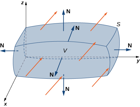
Figure 1. The divergence theorem relates a flux integral across a closed surface [latex]S[/latex] to a triple integral over solid [latex]E[/latex] enclosed by the surface.

Recall that the flux form of Green’s theorem states that [latex]\displaystyle\iint_D\text{div }{\bf{F}}dA=\displaystyle\int_C{\bf{F}}\cdot{\bf{N}}ds[/latex]. Therefore, the divergence theorem is a version of Green’s theorem in one higher dimension.

The proof of the divergence theorem is beyond the scope of this text. However, we look at an informal proof that gives a general feel for why the theorem is true, but does not prove the theorem with full rigor. This explanation follows the informal explanation given for why Stokes’ theorem is true.

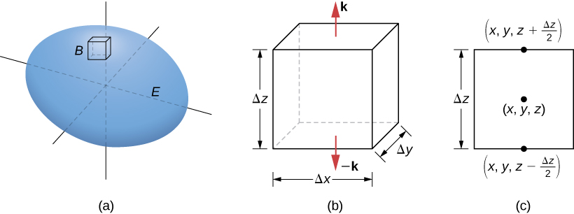
Figure 2. (a) A small box [latex]B[/latex] inside surface [latex]E[/latex] has sides parallel to the coordinate planes. (b) Box [latex]B[/latex] has side lengths [latex]{\Delta x}[/latex],[latex]{\Delta y}[/latex], and [latex]{\Delta z}[/latex] (c) If we look at the side view of [latex]B[/latex], we see that, since [latex](x, y, z)[/latex] is the center of the box, to get to the top of the box we must travel a vertical distance of [latex]{\Delta z}/2[/latex] up from [latex](x, y, z)[/latex]. Similarly, to get to the bottom of the box we must travel a distance [latex]{\Delta z}/2[/latex] down from [latex](x, y, z)[/latex].

The flux out of the top of the box can be approximated by [latex]R\left(x,y,z+\frac{\Delta z}{2}\right)\Delta x\Delta y[/latex] (Figure 2(c)) and the flux out of the bottom of the box is [latex]-R\left(x,y,z-\frac{\Delta z}{2}\right)\Delta x\Delta y[/latex]. If we denote the difference between these values as [latex]\Delta R[/latex], then the net flux in the vertical direction can be approximated by [latex]\Delta R\Delta x\Delta y[/latex]. However,

[latex]\large{\Delta R\Delta x\Delta y=\left(\frac{\Delta R}{\Delta z}\right)\Delta x\Delta y\Delta z\approx\left(\frac{\partial R}{\partial z}\right)\Delta V}[/latex].

Therefore, the net flux in the vertical direction can be approximated by [latex]\left(\frac{\partial R}{\partial z}\right)\Delta V[/latex]. Similarly, the net flux in the [latex]x[/latex]-direction can be approximated by [latex]\left(\frac{\partial P}{\partial x}\right)\Delta V[/latex] and the net flux in the [latex]y[/latex]-direction can be approximated by [latex]\left(\frac{\partial Q}{\partial y}\right)\Delta V[/latex]. Adding the fluxes in all three directions gives an approximation of the total flux out of the box:

Total flux [latex]\approx\left(\frac{\partial P}{\partial x}+\frac{\partial Q}{\partial y}+\frac{\partial R}{\partial z}\right)\Delta V=\text{div }{\bf{F}}\Delta V[/latex].

This approximation becomes arbitrarily close to the value of the total flux as the volume of the box shrinks to zero.

The sum of [latex]\text{div }{\bf{F}}\Delta V[/latex] over all the small boxes approximating [latex]E[/latex] is approximately [latex]\displaystyle\iiint_E\text{div }{\bf{F}}dV[/latex]. On the other hand, the sum of [latex]\text{div }{\bf{F}}\Delta V[/latex] over all the small boxes approximating [latex]E[/latex] is the sum of the fluxes over all these boxes. Just as in the informal proof of Stokes’ theorem, adding these fluxes over all the boxes results in the cancelation of a lot of the terms. If an approximating box shares a face with another approximating box, then the flux over one face is the negative of the flux over the shared face of the adjacent box. These two integrals cancel out. When adding up all the fluxes, the only flux integrals that survive are the integrals over the faces approximating the boundary of [latex]E[/latex]. As the volumes of the approximating boxes shrink to zero, this approximation becomes arbitrarily close to the flux over [latex]S[/latex].

[latex]_\blacksquare[/latex]

Example: verifying the divergence theorem

Verify the divergence theorem for vector field [latex]{\bf{F}}=\langle x-y,x+z, z-y\rangle[/latex] and surface [latex]S[/latex] that consists of cone [latex]x^{2}+y^{2}=z^{2}[/latex], [latex]0\leq z\leq1[/latex], and the circular top of the cone (see the following figure). Assume this surface is positively oriented.

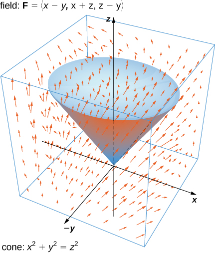
Figure 3. The vector field [latex]{\bf{F}}=\langle x-y,x+z, z-y\rangle[/latex] and surface [latex]S[/latex] that consists of cone [latex]x^{2}+y^{2}=z^{2}[/latex], [latex]0\leq z\leq1[/latex], and the circular top of the cone

Show Solution

Let [latex]E[/latex] be the solid cone enclosed by [latex]S[/latex]. To verify the theorem for this example, we show that [latex]\displaystyle\iiint_E\text{div }{\bf{F}}dV=\displaystyle\iint_s{\bf{F}}\cdot d{\bf{S}}[/latex] by calculating each integral separately.

To compute the triple integral, note that [latex]\text{div }{\bf{F}}=P_x+Q_y+R_z=2[/latex], and therefore the triple integral is

[latex]\large{\begin{aligned} \displaystyle\iiint_E\text{div }{\bf{F}}dV&=2\displaystyle\iiint_EdV \\ &=2\text{(volume of E)} \end{aligned}}[/latex].

The volume of a right circular cone is given by [latex]\pi{r}^2\frac{h}3[/latex]. In this case, [latex]h=r=1[/latex]. Therefore,

[latex]\large{\displaystyle\iiint_E\text{div }{\bf{F}}dV=2}\text{(volume of E)}=\frac{2\pi}{3}[/latex].

To compute the flux integral, first note that [latex]S[/latex] is piecewise smooth; [latex]S[/latex] can be written as a union of smooth surfaces. Therefore, we break the flux integral into two pieces: one flux integral across the circular top of the cone and one flux integral across the remaining portion of the cone. Call the circular top [latex]S_1[/latex] and the portion under the top [latex]S_2[/latex]. We start by calculating the flux across the circular top of the cone. Notice that [latex]S_1[/latex] has parameterization

[latex]\large{{\bf{r}}(u,v)=\langle u,\cos v,u\sin v,1\rangle, \ 0\leq u\leq1, \ 0\leq v\leq2\pi}[/latex].

Then, the tangent vectors are [latex]{\bf{t}}_u\langle\cos v,\sin v, 0\rangle[/latex] and [latex]{\bf{t}}_v=\langle-u\cos v,u\sin v,0\rangle[/latex]. Therefore, the flux across [latex]S_1[/latex] is

[latex]\begin{aligned} \displaystyle\iint_{S_1}{\bf{F}}\cdot d{\bf{S}}&=\displaystyle\int_0^1\displaystyle\int_0^{2\pi}{\bf{F}}({\bf{r}}(u,v))\cdot({\bf{t}}_u\times{\bf{t}}_v)dA \\ &=\displaystyle\int_0^1\displaystyle\int_0^{2\pi}\langle u\cos v-u\sin v,u\cos v+1,1-u\sin v\rangle\cdot\langle0,0,u\rangle \ dvdu \\ &=\displaystyle\int_0^1\displaystyle\int_0^{2\pi}u-u^2\sin v \ dvdu=\pi \end{aligned}[/latex].

We now calculate the flux over [latex]S_2[/latex]. A parameterization of this surface is

[latex]\large{{\bf{r}}(u,v)=\langle u,\cos v,u\sin v,1\rangle, \ 0\leq u\leq1, \ 0\leq v\leq2\pi}[/latex].

The tangent vectors are [latex]{\bf{t}}_u\langle\cos v,\sin v, 1\rangle[/latex] and [latex]{\bf{t}}_v\langle-u\sin v,u\cos v, 0\rangle[/latex], so the cross product is

[latex]\large{{\bf{t}}_u\times{\bf{t}}_v=\langle-u\cos v, -\sin v, u\rangle}[/latex].

Notice that the negative signs on the [latex]x[/latex] and [latex]y[/latex] components induce the negative (or inward) orientation of the cone. Since the surface is positively oriented, we use vector [latex]{\bf{t}}_u\times{\bf{t}}_v=\langle u\cos v,u\sin v,-u\rangle[/latex] in the flux integral. The flux across [latex]S_2[/latex] is then

[latex]\begin{aligned} \displaystyle\iint_{S_2}{\bf{F}}\cdot d{\bf{S}}&=\displaystyle\int_0^1\displaystyle\int_0^{2\pi}{\bf{F}}({\bf{r}}(u,v))\cdot({\bf{t}}_u\times{\bf{t}}_v)dA \\ &=\displaystyle\int_0^1\displaystyle\int_0^{2\pi}\langle u\cos v-u\sin v,u\cos v+u,u-u\sin v\rangle\cdot\langle u\cos v,u\sin v,-u\rangle \\ &=\displaystyle\int_0^1\displaystyle\int_0^{2\pi}u^2\cos^2v+2u^2\sin v-u^2 \ dvdu=-\frac{\pi}3 \end{aligned}[/latex].

The total flux across [latex]S[/latex] is

[latex]\large{\displaystyle\iint_{S_2}{\bf{F}}\cdot d{\bf{S}}=\displaystyle\iint_{S_1}{\bf{F}}\cdot d{\bf{S}}+\displaystyle\iint_{S_2}{\bf{F}}\cdot d{\bf{S}}=\frac{2\pi}3=\displaystyle\iiint_e\text{div }{\bf{F}}dV}[/latex],

and we have verified the divergence theorem for this example.

Watch the following video to see the worked solution to the above Try It

Recall that the divergence of continuous field [latex]{\bf{F}}[/latex] at point [latex]P[/latex] is a measure of the “outflowing-ness” of the field at [latex]P[/latex]. If [latex]{\bf{F}}[/latex] represents the velocity field of a fluid, then the divergence can be thought of as the rate per unit volume of the fluid flowing out less the rate per unit volume flowing in. The divergence theorem confirms this interpretation. To see this, let [latex]P[/latex] be a point and let [latex]B_r[/latex] be a ball of small radius [latex]r[/latex] centered at [latex]P[/latex] (Figure 4). Let [latex]S_r[/latex] be the boundary sphere of [latex]B_r[/latex]. Since the radius is small and [latex]{\bf{F}}[/latex] is continuous, [latex]\text{div }{\bf{F}}(Q)\approx\text{div }{\bf{F}}(P)[/latex] for all other points [latex]Q[/latex] in the ball. Therefore, the flux across [latex]S_r[/latex] can be approximated using the divergence theorem:

[latex]\large{\displaystyle\iint_{S_r}{\bf{F}}\cdot dS=\displaystyle\iiint_{B_r}\text{div }{\bf{F}}dV\approx\displaystyle\iiint_{B_r}\text{div }{\bf{F}}(P)dV}[/latex].

Since [latex]\text{div }{\bf{F}}(P)[/latex] is a constant,

[latex]\large{\displaystyle\iiint_{B_r}\text{div }{\bf{F}}(P)dV=\text{div }{\bf{F}}(P)V(B_r)}[/latex].

Therefore, flux [latex]\displaystyle\iint_{S_r}{\bf{F}}\cdot d{\bf{S}}[/latex] can be approximated by [latex]\text{div }{\bf{F}}(P)V(B_r)[/latex]. This approximation gets better as the radius shrinks to zero, and therefore

[latex]\large{\text{div }{\bf{F}}(P)=\displaystyle\lim_{r\to0}\frac{1}{V(B_r)}\displaystyle\iint_{S_r}{\bf{F}}\cdot d{\bf{S}}}[/latex].

This equation says that the divergence at [latex]P[/latex] is the net rate of outward flux of the fluid per unit volume.

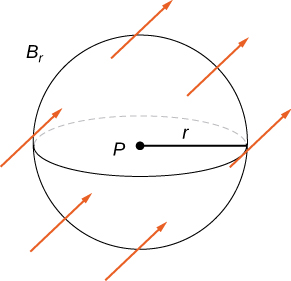
Figure 4. Ball [latex]B_r[/latex] of small radius [latex]r[/latex] centered at [latex]P[/latex].