Working with Vectors in Three Dimensions

Learning Objectives

Perform vector operations in [latex]\mathbb{R}^3[/latex].

Just like two-dimensional vectors, three-dimensional vectors are quantities with both magnitude and direction, and they are represented by directed line segments (arrows). With a three-dimensional vector, we use a three-dimensional arrow.

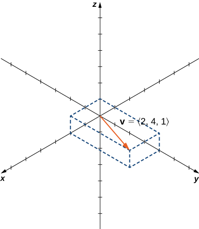
Three-dimensional vectors can also be represented in component form. The notation [latex]\mathbf{v} = \langle x,y,z \rangle[/latex] is a natural extension of the two-dimensional case, representing a vector with the initial point at the origin, [latex](0, 0, 0)[/latex], and terminal point [latex](x, y, z)[/latex]. The zero vector is [latex]\mathbf{0} = \langle 0,0,0 \rangle[/latex]. So, for example, the three dimensional vector [latex]\mathbf{v} = \langle 2,4,1 \rangle[/latex] is represented by a directed line segment from point [latex](0, 0, 0)[/latex] to point [latex](2, 4, 1)[/latex] (Figure 1).

This figure is the 3-dimensional coordinate system. It has a vector drawn. The initial point of the vector is the origin. The terminal point of the vector is (2, 4, 1). The vector is labeled “v = <2, 4, 1>.”

Figure 1. Vector [latex]v=⟨2,4,1⟩[/latex] is represented by a directed line segment from point [latex](0,0,0)[/latex] to point [latex](2,4,1)[/latex].

Vector addition and scalar multiplication are defined analogously to the two-dimensional case. If [latex]\mathbf{v} = \langle x_1,y_1,z_1 \rangle[/latex] and [latex]\mathbf{w} = \langle x_2,y_2,z_2 \rangle[/latex] are vectors, and [latex]k[/latex] is a scalar, then

[latex]\mathbf{v+w} = \langle x_1 + x_2,y_1 + y_2,z_1 +z_2 \rangle[/latex] and [latex]k\mathbf{v} = \langle k x_1,k y_1,k z_1 \rangle.[/latex]

If [latex]k=-1[/latex], then [latex]k\mathbf{v} = (-1)\mathbf{v} [/latex] is written as [latex]-\mathbf{v} [/latex], and vector subtraction is defined by [latex]\mathbf{v-w} = \mathbf{v+ (-w)} = \mathbf{v} + (-1)\mathbf{w} [/latex].

The standard unit vectors extend easily into three dimensions as well—[latex]\mathbf{i} = \langle 1,0,0 \rangle[/latex], [latex]\mathbf{j} = \langle 0,1,0 \rangle[/latex], and [latex]\mathbf{k} = \langle 0,0,1 \rangle[/latex]—and we use them in the same way we used the standard unit vectors in two dimensions. Thus, we can represent a vector in [latex]\mathbb{R}^3[/latex] in the following ways:

[latex]\mathbf{v} = \langle x,y,z \rangle = x\mathbf{i} + y\mathbf{j} + z\mathbf{k}[/latex].

Example: vector representations

Let [latex]\overrightarrow{PQ}[/latex] be the vector with initial point [latex]P=(3, 12, 6)[/latex] and terminal point [latex]Q=(-4, -3, 2)[/latex] as shown in Figure 2. Express [latex]\overrightarrow{PQ}[/latex] in both component form and using standard unit vectors.

This figure is the 3-dimensional coordinate system. It has two points labeled. The first point is P = (3, 12, 6). The second point is Q = (-4, -3, 2). There is a vector from P to Q.

Figure 2. The vector with initial point [latex]P=(3,12,6)[/latex] and terminal point [latex]Q=(−4,−3,2)[/latex].

Show Solution

try it

Let [latex]S=(3, 8, 2)[/latex] and [latex]T=(2, -1, 3)[/latex]. Express [latex]\overrightarrow{ST}[/latex] in component form and in standard unit form.

Show Solution

As described earlier, vectors in three dimensions behave in the same way as vectors in a plane. The geometric interpretation of vector addition, for example, is the same in both two- and three-dimensional space (Figure 3).

This figure is the first octant of the 3-dimensional coordinate system. It has has three vectors in standard position. The first vector is labeled “A.” The second vector is labeled “B.” The third vector is labeled “A + B.” This vector is in between vectors A and B.

Figure 3. To add vectors in three dimensions, we follow the same procedures we learned for two dimensions.

We have already seen how some of the algebraic properties of vectors, such as vector addition and scalar multiplication, can be extended to three dimensions. Other properties can be extended in similar fashion. They are summarized here for our reference.

rule: properties of vectors in space

Let [latex]\mathbf{v} = \langle x_1,y_1,z_1 \rangle[/latex] and [latex]\mathbf{w} = \langle x_2,y_2,z_2 \rangle[/latex] be vectors, and let [latex]k[/latex] be a scalar.
Scalar multiplication: [latex]k\mathbf{v} = \langle kx_1,ky_1,kz_1 \rangle[/latex]
Vector addition: [latex]\mathbf{v+ w} = \langle x_1,y_1,z_1 \rangle + \langle x_2,y_2,z_2 \rangle = \langle x_1 +x_2,y_1 +y_2,z_1 +z_2 \rangle[/latex]
Vector subtraction: [latex]\mathbf{v- w} = \langle x_1,y_1,z_1 \rangle - \langle x_2,y_2,z_2 \rangle = \langle x_1 -x_2,y_1 -y_2,z_1 -z_2 \rangle[/latex]
Vector magnitude: [latex]\|\mathbf{v}\| = \sqrt{x_1^2 + y_1 ^2 + z_1 ^2}[/latex]
Unit vector in the direction of v: [latex]\frac{1}{\|\mathbf{v}\|}\mathbf{v} = \frac{1}{\|\mathbf{v}\|} \langle x_1,y_1,z_1 \rangle = \langle \frac{x_1}{\|\mathbf{v}\|}\frac{y_1}{\|\mathbf{v}\|}\frac{z_1}{\|\mathbf{v}\|} \rangle[/latex] if [latex]\mathbf{v} \neq \mathbf{0}[/latex].

We have seen that vector addition in two dimensions satisfies the commutative, associative, and additive inverse properties. These properties of vector operations are valid for three-dimensional vectors as well. Scalar multiplication of vectors satisfies the distributive property, and the zero vector acts as an additive identity. The proofs to verify these properties in three dimensions are straightforward extensions of the proofs in two dimensions.

Example: vector operations in three dimensions

Let [latex]\mathbf{v} = \langle -2,9,5 \rangle[/latex] and [latex]\mathbf{w} = \langle 1,-1,0 \rangle[/latex] (Figure 4). Find the following vectors.

[latex]3\mathbf{v} -2\mathbf{w}[/latex]
[latex]5\|\mathbf{w}\|[/latex]
[latex]\|5\mathbf{w}\|[/latex]
A unit vector in the direction of [latex]\textbf v[/latex]

This figure is the 3-dimensional coordinate system. It has two vectors in standard position. The first vector is labeled “v = <-2, 9, 5>.” The second vector is labeled “w = <1, -1, 0>.”

Figure 4. The vectors [latex]{\bf{v}}=⟨−2,9,5⟩[/latex] and [latex]{\bf{w}}=⟨1,−1,0⟩[/latex].

Show Solution

try it

Let [latex]\mathbf{v} = \langle -1,-1,1 \rangle[/latex] and [latex]\mathbf{w} = \langle 2,0,1 \rangle[/latex]. Find a unit vector in the direction of [latex]5\mathbf{v}+3\mathbf{w}[/latex].

Show Solution

Watch the following video to see the worked solution to the above Try IT.

You can view the transcript for “CP 2.19” here (opens in new window)

Try It

Example: throwing a forward pass

A quarterback is standing on the football field preparing to throw a pass. His receiver is standing 20 yd down the field and 15 yd to the quarterback’s left. The quarterback throws the ball at a velocity of 60 mph toward the receiver at an upward angle of [latex]30^\circ[/latex] (see the following figure). Write the initial velocity vector of the ball, [latex]\textbf v[/latex], in component form.

This figure is an image of two football players with the first one throwing the football to the second one. There is a line segment from each player to the bottom of the image. The distance from the first player to the bottom of the image is 20 yards. The distance from the second player to the same point on the bottom of the image is 15 yards. The two line segments are perpendicular. There is a broken line segment from the first player to the second player. There is a vector from the first player. The angle between the broken line and the vector is 30 degrees.

Figure 5. The receiver is standing [latex]20[/latex] yd down the field and [latex]15[/latex] yd to the quarterback’s left. The quarterback throws the ball at a velocity of [latex]60[/latex] mph toward the receiver at an upward angle of [latex]30°[/latex]

Show Solution

The first thing we want to do is find a vector in the same direction as the velocity vector of the ball. We then scale the vector appropriately so that it has the right magnitude. Consider the vector [latex]\textbf w[/latex] extending from the quarterback’s arm to a point directly above the receiver’s head at an angle of [latex]30^\circ[/latex] (see the following figure). This vector would have the same direction as [latex]\textbf v[/latex], but it may not have the right magnitude.

This figure is the image of two football players with the first player throwing the football to the second player. The distance between the two players is represented with a broken line segment. There is a vector from the first player. The angle between the vector and the broken line segment is 30 degrees. There is a vertical broken line segment from the second player. Also, there is a right triangle formed from the two broken line segments and the vector from the first player is labeled “w” and is the hypotenuse.

Figure 6. Vector [latex]{\bf{w}}[/latex] extending from the quarterback’s arm at an angle of [latex]30°[/latex]

The receiver is 20 yd down the field and 15 yd to the quarterback’s left. Therefore, the straight-line distance from the quarterback to the receiver is

[latex]\text{Dist from QB to receiver} = \sqrt{15^2 + 20^2} = \sqrt{225 + 400} = \sqrt{625} = 25 [/latex] yd.

We have [latex]\frac{25}{\|\mathbf{w}\|} = \cos{30^\circ}[/latex]. Then the magnitude of [latex]\textbf w[/latex] is given by

[latex]\|\mathbf{w}\| = \frac{25}{\cos{30^\circ}} = \frac{25*2}{\sqrt{3}} = \frac{50}{\sqrt{3}}[/latex]yd

and the vertical distance from the receiver to the terminal point of [latex]\textbf w[/latex] is

[latex]\text{Vert dist from receiver to terminal point of } \textbf w = \textbf w \sin{30^\circ} = \frac{50}{\sqrt{3}} * \frac{1}{2} = \frac{25}{\sqrt{3}} [/latex]yd.

Then [latex]\mathbf{w} = \langle 20,15,\frac{25}{\sqrt{3}} \rangle[/latex], and has the same direction as [latex]\textbf v[/latex].

Recall, though, that we calculated the magnitude of [latex]\textbf w[/latex]to be [latex]\|\textbf w\| = \frac{50}{\sqrt{3}}[/latex], and [latex]\textbf v[/latex] has magnitude 60 mph. So, we need to multiply vector [latex]\textbf w[/latex] by an appropriate constant, [latex]k[/latex]. We want to find a value of [latex]k[/latex] so that [latex]\|k \textbf{w}\| = 60[/latex] mph. We have

[latex]\|k \textbf{w} \|= k \|\textbf{w}\| = k\frac{50}{\sqrt{3}} [/latex] mph,

so we want

[latex] \begin{align*} k\frac{50}{\sqrt{3}} &= 60 \\ k &= \frac{60\sqrt{3}}{50}\\ k &= \frac{6\sqrt{3}}{5}\\ \end{align*} [/latex].

Then

[latex]\textbf{v} = k\textbf{w} = k \langle 20,15,\frac{25}{\sqrt{3}} \rangle= \frac{6\sqrt{3}}{5}\langle 20,15,\frac{25}{\sqrt{3}}\rangle = \langle 24\sqrt{3},18\sqrt{3},30\rangle [/latex].

Let’s double-check that [latex]\|\textbf{v}\|=60[/latex]. We have

[latex]\|\textbf{v}\| = \sqrt{(24\sqrt{3})^2+(18\sqrt{3})^2+(30)^2} = \sqrt{1728+972+900} = \sqrt{3600} = 60 [/latex]mph.

So, we have found the correct components for [latex]\textbf v[/latex].

try it

Assume the quarterback and the receiver are in the same place as in the previous example. This time, however, the quarterback throws the ball at velocity of 40 mph and an angle of [latex]45^\circ[/latex]. Write the initial velocity vector of the ball, [latex]\textbf v[/latex], in component form.

Show Solution

Module 2: Vectors in Space