Introduction
What you’ll learn to do: Make calculations and predictions using explicit equations for both linear and exponential growth
Constant change is the defining characteristic of linear growth. Plotting coordinate pairs associated with constant change will result in a straight line, the shape of linear growth. In this section, we will formalize a way to describe linear growth using mathematical terms and concepts. By the end of this section, you will be able to recognize the difference between linear and exponential growth given a graph or an equation.

Learning Outcomes
- Determine whether given data or scenarios describe linear growth
- Identify growth rates, initial values, or point values expressed verbally, graphically, or numerically, and translate them into a format usable in calculation
- Calculate equations for linear growth and use those equations to make predictions
- Determine whether given data or scenarios describe linear or exponential growth
- Identify growth rates, initial values, or point values expressed verbally, graphically, or numerically, and translate them into a format usable in calculation
- Use equations for exponential growth to make predictions
Linear Growth
Marco is a collector of antique soda bottles. His collection currently contains 437 bottles. Every year, he budgets enough money to buy 32 new bottles. Can we determine how many bottles he will have in 5 years, and how long it will take for his collection to reach 1000 bottles?

While you may be able to answer both of these questions without an equation or formal mathematics, we are going to formalize our approach to this problem to provide a means to answer more complicated questions.
Let’s try to create a problem solving pathway to determine how many bottles Marco will have in 5 years.
- To find out how many bottles Marco will have in five years, we need to add the number of bottles currently in his collection to the number of new bottles he will gain over five years.
- To determine how many new bottles will be added to his current collection over 5 years, we need to know how many will be added each year and multiply by 5.
Working backwards through out pathway, we have:
Step 2: Marco will gain 32 bottles per year for each of 5 years: [latex]\displaystyle\frac{32 \text{ bottles}}{\text{year}} \cdot 5 \text{ years}=160 \text{ bottles}[/latex]; Marco will add 160 bottles to his collection in 5 years.
Step 1: Marco has 437 bottles currently, so we add this to the number of bottles gained in 5 years: [latex]437 + 160=597[/latex]; Marco will have 597 bottles in his collection after five years. This answers our first question.
Now, to find when Marco will have 1000 bottles, we can create a formula using the method above. Instead of 5 years, we will calculate a formula for the number of bottles after [latex]n[/latex] years.
Step 2: Marco will gain 32 bottles per year for each of [latex]n[/latex] years: [latex]\displaystyle\frac{32 \text{ bottles}}{\text{year}} \cdot n \text{ years}=32n \text{ bottles}[/latex]; Marco will add [latex]32n[/latex] bottles to his collection in [latex]n[/latex] years.
Step 1: Marco has 437 bottles currently, so we add this to the number of bottles gained in [latex]n[/latex] years: [latex]437 + 32n=[/latex] the number of bottles in his collection after [latex]n[/latex] years. So we might write the formula [latex]437 + 32n= P_n[/latex] where [latex]P_n[/latex] is the number of bottles in the collections after [latex]n[/latex] years.
To answer our second question, we need [latex]P_n[/latex] to equal 1000. So we solve the equation [latex]1000 = 437 + 32n[/latex] to obtain [latex]n\approx17.59[/latex] years. Therefore, we might estimate that it will take Marco 18 years to have 1000 bottles.
recall translating between words and mathematical operations
In the description above, the desired equation is built up by describing and translating between math notation and words. If you read the lines in words as you go, it may help reveal what’s being done.
Ex. [latex]P_n=437+32n[/latex] may be read, “In n years, the number of bottles in the collection is the sum of the initial number of 437 bottles plus 32n additional bottles”.
Translating between the real-world situation and the mathematical notation as you work through an example can help you to understand the process being used to create the explicit equation that describes the situation.
In the previous example, Marco’s collection grew by the same number of bottles every year. This constant change is the defining characteristic of linear growth. Plotting the values we calculated for Marco’s collection, we can see the values form a straight line, the shape of linear growth.
Linear Growth
If a quantity starts at size [latex]P_0[/latex] and grows by [latex]d[/latex] every time period, then the quantity after [latex]n[/latex] time periods can be determined using the following equation:
[latex]P_n = P_0 +dn[/latex]
In this equation, [latex]d[/latex] represents the common difference – the amount that the population changes each time [latex]n[/latex] increases by 1.
Connection to Prior Learning: Slope and Intercept
You may recognize the common difference, [latex]d[/latex], in our linear equation as slope. In fact, the entire explicit equation should look familiar – it is the same linear equation you learned in algebra, probably stated as [latex]y = mx + b[/latex].
In the standard algebraic equation [latex]y = mx + b, b[/latex] was the [latex]y[/latex]-intercept, or the [latex]y[/latex] value when [latex]x[/latex] was zero. In the form of the equation we’re using, we are using [latex]P_0[/latex] to represent that initial amount.
In the [latex]y = mx + b[/latex] equation, recall that [latex]m[/latex] was the slope. You might remember this as “rise over run,” or the change in [latex]y[/latex] divided by the change in [latex]x[/latex]. Either way, it represents the same thing as the common difference, [latex]d[/latex], we are using – the amount the output [latex]P_n[/latex] changes when the input [latex]n[/latex] increases by 1.
The equations [latex]y = mx + b[/latex] and [latex]P_n = P_0 +dn[/latex] mean the same thing and can be used the same ways. We’re just writing it a little differently.
Examples
Example 1: The population of elk in a national forest was measured to be 12,000 in 2003, and was measured again to be 15,000 in 2007. If the population continues to grow linearly at this rate, what will the elk population be in 2014?
This example is worked out in the following video. Note that 43 seconds into the video, the presenter briefly mentions a “recursive” model–you may safely ignore this phrase since we have omitted this type of model from our course discussion.
Example 2: The cost, in dollars, of a gym membership for n months can be described by the explicit equation [latex]P_n = 70 + 30n[/latex]. What does this equation tell us?
The explanation for this example is detailed in the video below.
Try It
All of the examples we have considered so far in this section describe situations that are precisely linear. That is, the output (“number of new bottles” or “number of elk” or “cost of gym membership”) changes by exactly the same amount each time period. However, real world data rarely fall precisely on a line (i.e.: the output rarely changes by exactly the same amount each time period). Yet it is often the case that data are close to being linear. In the next example, we investigate how to solve problems in which we have data that we recognize as being “almost linear.”
Example
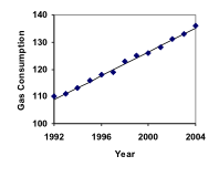
Gasoline consumption in the US has been increasing steadily. Gasoline consumption data from 1992 to 2004 are shown below.[1]
| Year | ’92 | ’93 | ’94 | ’95 | ’96 | ’97 | ’98 | ’99 | ’00 | ’01 | ’02 | ’03 | ’04 |
| Consumption (billion of gallons) | 110 | 111 | 113 | 116 | 118 | 119 | 123 | 125 | 126 | 128 | 131 | 133 | 136 |
- Find a model for these data, and use it to predict consumption in 2016.
- If the trend continues, when do you predict gasoline consumption to reach 200 billion gallons?

The steps for reaching this answer are detailed in the following video.
When Good Models Go Bad
When using mathematical models to predict future behavior, it is important to keep in mind that very few trends will continue indefinitely.
Example
Suppose a four year old boy is currently 39 inches tall, and you are told to expect him to grow 2.5 inches a year. We can set up a growth model, with [latex]n[/latex] defined to be the number of years past 4 (years old). That is, [latex]n = 0[/latex] corresponds to when the child is 4 years old. Thus, [latex]P_0 = 39[/latex] inches and [latex]d = 2.5[/latex] inches per year giving us the model:
[latex]P_n = 39 + 2.5n[/latex]
So at 6 years old, we would expect him to be: [latex]P_2 = 39 + 2.5(2) = 44[/latex] inches tall
Of course, we wouldn’t expect this boy to continue to grow at the same rate all his life. If he did, at age 50 he would be [latex]P_{46} = 39 + 2.5(46) = 154[/latex] inches tall. That’s 12.8 feet tall!
Important Idea: When using any mathematical model, we have to consider which inputs are reasonable to use. Whenever we make predictions into the future (the mathematical word for this is we extrapolate), we are making an assumption that the model will continue to be valid. We must take care to ensure that this is indeed a reasonable assumption to make.
View a video explanation of this breakdown of the linear growth model here.
Candela Citations
- Revision and Adaptation. Provided by: Lumen Learning. License: CC BY: Attribution
- Linear (Algebraic) Growth. Authored by: David Lippman. Located at: http://www.opentextbookstore.com/mathinsociety/. Project: Math in Society. License: CC BY-SA: Attribution-ShareAlike
- Feira Tom Jobim - BH. Authored by: Antonio Thomas Koenigkam Oliveira. Located at: https://flic.kr/p/p8ZqqF. License: CC BY: Attribution
- Linear Growth Part 1. Authored by: OCLPhase2's channel. Located at: https://youtu.be/SJcAjN-HL_I. License: CC BY: Attribution
- Linear Growth Part 2. Authored by: OCLPhase2's channel. Located at: https://youtu.be/4Two_oduhrA. License: CC BY: Attribution
- Linear Growth Part 3. Authored by: OCLPhase2's channel. Located at: https://youtu.be/pZ4u3j8Vmzo. License: CC BY: Attribution
- Linear Growth - Elk. Authored by: OCLPhase2's channel. Located at: https://youtu.be/J1XqqlKzYGs. License: CC BY: Attribution
- Finding linear model for gas consumption. Authored by: OCLPhase2's channel. Located at: https://youtu.be/ApFxDWd6IbE. License: CC BY: Attribution
- Interpreting a linear model. Authored by: OCLPhase2's channel. Located at: https://youtu.be/0Uwz5dmLTtk. License: CC BY: Attribution
- Linear model breakdown. Authored by: OCLPhase2's channel. Located at: https://youtu.be/6zfXCsmcDzI. License: CC BY: Attribution
- Question ID 6594. Authored by: Lippman,David. License: CC BY: Attribution. License Terms: IMathAS Community License CC-BY + GPL