Figure 1. A nuclear research reactor inside the Neely Nuclear Research Center on the Georgia Institute of Technology campus (credit: Georgia Tech Research Institute)

Because the output of exponential functions increases very rapidly, the term “exponential growth” is often used in everyday language to describe anything that grows or increases rapidly. However, exponential growth can be defined more precisely in a mathematical sense. If the growth rate is proportional to the amount present, the function models exponential growth.

In more general terms, we have an exponential function, in which a constant base is raised to a variable exponent. To differentiate between linear and exponential functions, let’s consider two companies, A and B. Company A has 100 stores and expands by opening 50 new stores a year, so its growth can be represented by the function [latex]A\left(x\right)=100+50x[/latex]. Company B has 100 stores and expands by increasing the number of stores by 50% each year, so its growth can be represented by the function [latex]B\left(x\right)=100{\left(1+0.5\right)}^{x}[/latex].

A few years of growth for these companies are illustrated below.

The graphs comparing the number of stores for each company over a five-year period are shown in below. We can see that, with exponential growth, the number of stores increases much more rapidly than with linear growth.

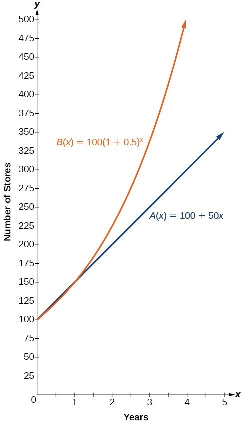
Figure 2. The graph shows the numbers of stores Companies A and B opened over a five-year period.

Notice that the domain for both functions is [latex]\left[0,\infty \right)[/latex], and the range for both functions is [latex]\left[100,\infty \right)[/latex]. After year 1, Company B always has more stores than Company A.

Now we will turn our attention to the function representing the number of stores for Company B, [latex]B\left(x\right)=100{\left(1+0.5\right)}^{x}[/latex]. In this exponential function, 100 represents the initial number of stores, 0.50 represents the growth rate, and [latex]1+0.5=1.5[/latex] represents the growth factor. Generalizing further, we can write this function as [latex]B\left(x\right)=100{\left(1.5\right)}^{x}[/latex], where 100 is the initial value, 1.5 is called the base, and x is called the exponent.

 Find the Equation of an Exponential Function

In the previous examples, we were given an exponential function, which we then evaluated for a given input. Sometimes we are given information about an exponential function without knowing the function explicitly. We must use the information to first write the form of the function, then determine the constants a and b, and evaluate the function.

How To: Given two data points, write an exponential model.

1. If one of the data points has the form [latex]\left(0,a\right)[/latex], then a is the initial value. Using a, substitute the second point into the equation [latex]f\left(x\right)=a{\left(b\right)}^{x}[/latex], and solve for b.
2. If neither of the data points have the form [latex]\left(0,a\right)[/latex], substitute both points into two equations with the form [latex]f\left(x\right)=a{\left(b\right)}^{x}[/latex]. Solve the resulting system of two equations in two unknowns to find a and b.
3. Using the a and b found in the steps above, write the exponential function in the form [latex]f\left(x\right)=a{\left(b\right)}^{x}[/latex].

Example 2: Writing an Exponential Model When the Initial Value Is Known

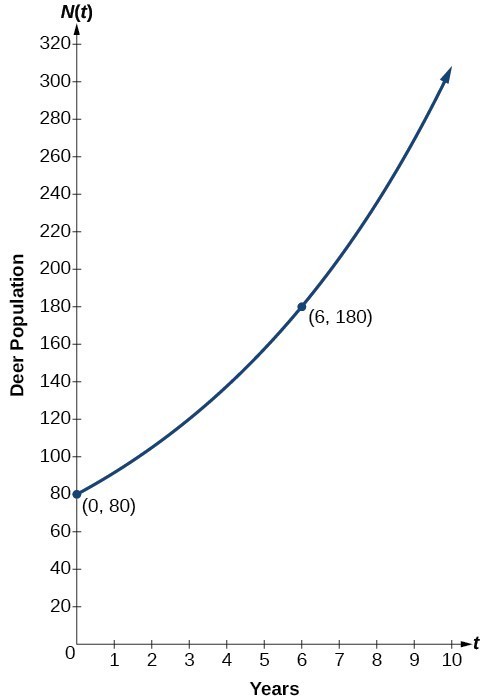
In 2006, 80 deer were introduced into a wildlife refuge. By 2012, the population had grown to 180 deer. The population was growing exponentially. Write an algebraic function N(t) representing the population N of deer over time t.

Show Solution

We let our independent variable t be the number of years after 2006. Thus, the information given in the problem can be written as input-output pairs: (0, 80) and (6, 180). Notice that by choosing our input variable to be measured as years after 2006, we have given ourselves the initial value for the function, a = 80. We can now substitute the second point into the equation [latex]N\left(t\right)=80{b}^{t}[/latex] to find b:

[latex]\begin{align}N\left(t\right)& =80{b}^{t} \\ 180& =80{b}^{6} && \text{Substitute using point }\left(6, 180\right). \\ \frac{9}{4} & ={b}^{6} && \text{Divide and write in lowest terms}. \\ b & ={\left(\frac{9}{4}\right)}^{\frac{1}{6}} && \text{Isolate }b\text{ using properties of exponents}. \\ b & \approx 1.1447 && \text{Round to 4 decimal places}. \end{align}[/latex]

NOTE: Unless otherwise stated, do not round any intermediate calculations. Then round the final answer to four places for the remainder of this section.

The exponential model for the population of deer is [latex]N\left(t\right)=80{\left(1.1447\right)}^{t}[/latex]. (Note that this exponential function models short-term growth. As the inputs gets large, the output will get increasingly larger, so much so that the model may not be useful in the long term.)

We can graph our model to observe the population growth of deer in the refuge over time. Notice that the graph below passes through the initial points given in the problem, [latex]\left(0,\text{ 8}0\right)[/latex] and [latex]\left(\text{6},\text{ 18}0\right)[/latex]. We can also see that the domain for the function is [latex]\left[0,\infty \right)[/latex], and the range for the function is [latex]\left[80,\infty \right)[/latex].

Figure 3. Graph showing the population of deer over time, [latex]N\left(t\right)=80{\left(1.1447\right)}^{t}[/latex], t years after 2006

Try It

A wolf population is growing exponentially. In 2011, 129 wolves were counted. By 2013 the population had reached 236 wolves. What two points can be used to derive an exponential equation modeling this situation? Write the equation representing the population N of wolves over time t.

Show Solution

[latex]\left(0,129\right)[/latex] and [latex]\left(2,236\right);N\left(t\right)=129{\left(\text{1}\text{.3526}\right)}^{t}[/latex]

Model exponential growth and decay

In real-world applications, we need to model the behavior of a function. In mathematical modeling, we choose a familiar general function with properties that suggest that it will model the real-world phenomenon we wish to analyze. In the case of rapid growth, we may choose the exponential growth function:

[latex]A(t)={A}_{0}{e}^{kt}[/latex]

where [latex]{A}_{0}[/latex] is equal to the value at time zero, e is Euler’s constant, and k is a positive constant that determines the rate (percentage) of growth. We may use the exponential growth function in applications involving doubling time, the time it takes for a quantity to double. Such phenomena as wildlife populations, financial investments, biological samples, and natural resources may exhibit growth based on a doubling time. In some applications, however, as we will see when we discuss the logistic equation, the logistic model sometimes fits the data better than the exponential model.

On the other hand, if a quantity is falling rapidly toward zero, without ever reaching zero, then we should probably choose the exponential decay model. Again, we have the form [latex]A(t)={A}_{0}{e}^{kt}[/latex] where [latex]{A}_{0}[/latex] is the starting value, and e is Euler’s constant. Now k is a negative constant that determines the rate of decay. We may use the exponential decay model when we are calculating half-life, or the time it takes for a substance to exponentially decay to half of its original quantity. We use half-life in applications involving radioactive isotopes.

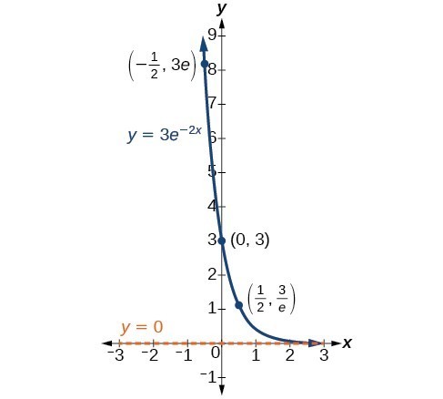
In our choice of a function to serve as a mathematical model, we often use data points gathered by careful observation and measurement to construct points on a graph and hope we can recognize the shape of the graph. Exponential growth and decay graphs have a distinctive shape, as we can see in Figure 4 and Figure 5. It is important to remember that, although parts of each of the two graphs seem to lie on the x-axis, they are really a tiny distance above the x-axis.

Exponential growth and decay often involve very large or very small numbers. To describe these numbers, we often use orders of magnitude. The order of magnitude is the power of ten, when the number is expressed in scientific notation, with one digit to the left of the decimal. For example, the distance to the nearest star, Proxima Centauri, measured in kilometers, is 40,113,497,200,000 kilometers. Expressed in scientific notation, this is [latex]4.01134972\times {10}^{13}[/latex]. So, we could describe this number as having order of magnitude [latex]{10}^{13}[/latex].

A General Note: Characteristics of the Exponential Function, [latex]y=A_{0}e^{kt}[/latex]

An exponential function with the form [latex]A(t)={A}_{0}{e}^{kt}[/latex] has the following characteristics:

• one-to-one function
• horizontal asymptote: y = 0
• domain: [latex]\left(-\infty , \infty \right)[/latex]
• range: [latex]\left(0,\infty \right)[/latex]
• x intercept: none
• y-intercept: [latex]\left(0,{A}_{0}\right)[/latex]
• increasing if k > 0
• decreasing if k < 0

Figure 6. An exponential function models exponential growth when k > 0 and exponential decay when k < 0.

Example 3: Exponential Growth

A population of bacteria doubles every hour. If the culture started with 10 bacteria, answer the following:

a) What is the exponential growth formula?
b) How many bacteria are present after 4 hours?
c) When will the population reach 640 bacteria?

Show Solution

a) When an amount grows at a fixed percent per unit time, the growth is exponential. To find [latex]{A}_{0}[/latex] we use the fact that [latex]{A}_{0}[/latex] is the amount at time zero, so [latex]{A}_{0}=10[/latex]. To find k, use the fact that after one hour [latex]\left(t=1\right)[/latex] the population doubles from 10 to 20. The formula is derived as follows

[latex]\begin{align}&20=10{e}^{k\cdot 1} \\ &2={e}^{k}&& \text{Divide by 10} \\ &\mathrm{ln}2=k&& \text{Take the natural logarithm} \end{align}[/latex]

so [latex]k=\mathrm{ln}\left(2\right)[/latex]. Thus the equation we want to graph is [latex]A(t)=10{e}^{\left(\mathrm{ln}2\right)t}=10{\left({e}^{\mathrm{ln}2}\right)}^{t}=10\cdot {2}^{t}[/latex].

b) To find the number of bacteria after 4 hours, we will substitute 4 in for t in our formula:  [latex]A(t)=10\cdot {2}^{t} \\A(4)=10\cdot {2}^{4} \\ A(4) = 160\text{ bacteria.}[/latex]
c) To find when the bacteria population will reach 640, we will substitute 640 for [latex]A(t)[/latex]: [latex]\text{ }A(t)=10\cdot {2}^{t} \\640=10\cdot {2}^{x} \\ 64={2}^{x} \\ x=6\text{ hours.}[/latex]

Example 4: Exponential Growth

At the start of an experiment, there are 100 cells. Three hours later, there were 250 cells. Answer the following:

a) What is the exponential growth formula?
b) How many bacteria are present after 4 hours?
c) When will the population reach 848 cells?

Show Solution

a) To find [latex]{A}_{0}[/latex] we use the fact that [latex]{A}_{0}[/latex] is the amount at time zero, so [latex]{A}_{0}=100[/latex]. To find k, use the fact that after three hours [latex]\left(t=3\right)[/latex] the population grows from 100 to 250. The formula is derived as follows

[latex]\begin{align}&250=100{e}^{k\cdot 3} \\ &2.5={e}^{3k}&& \text{Divide by 100} \\ &\mathrm{ln}(2.5)=3k&& \text{Take the natural logarithm} \end{align}[/latex]

so [latex]k=\dfrac{\mathrm{ln}\left(2.5\right)}{3}\approx 0.3054[/latex]. Thus the equation we want to graph is [latex]A(t)=100{e}^{0.3054t}[/latex].

b) To find the number of cells after 4 hours, we will substitute 4 in for t in our formula:  [latex]A(t)=100{e}^{0.3054t} \\ A(4)=100{e}^{0.3054(4)} \\ A(4)\approx 339\text{ cells.}[/latex]
c) To find when the bacteria population will reach 848, we will substitute 848 for [latex]A(t)[/latex]: [latex]A(t)=100{e}^{0.3054t} \\848=100{e}^{0.3054t} \\ 8.48={e}^{0.3054t} \\ t = \dfrac{\mathrm{ln}(8.48)}{0.3054}\approx 7\text{ hours.}[/latex]

Half-Life

In previous sections, we learned the properties and rules for both exponential and logarithmic functions. We have seen that any exponential function can be written as a logarithmic function and vice versa. We have used exponents to solve logarithmic equations and logarithms to solve exponential equations. We are now ready to combine our skills to solve equations that model real-world situations, whether the unknown is in an exponent or in the argument of a logarithm.

One such application is in science, in calculating the time it takes for half of the unstable material in a sample of a radioactive substance to decay, called its half-life. The table below lists the half-life for several of the more common radioactive substances.

Substance	Use	Half-life
gallium-67	nuclear medicine	80 hours
cobalt-60	manufacturing	5.3 years
technetium-99m	nuclear medicine	6 hours
americium-241	construction	432 years
carbon-14	archeological dating	5,715 years
uranium-235	atomic power	703,800,000 years

We can see how widely the half-lives for these substances vary. Knowing the half-life of a substance allows us to calculate the amount remaining after a specified time.

To find the half-life of a function describing exponential decay, solve the following equation:

[latex]\frac{1}{2}{A}_{0}={A}_{o}{e}^{kt}[/latex]

We find that the half-life depends only on the constant k and not on the starting quantity [latex]{A}_{0}[/latex].

The formula is derived as follows

[latex]\begin{align}\frac{1}{2}{A}_{0}&={A}_{o}{e}^{kt} \\ \frac{1}{2}&={e}^{kt}&& \text{Divide by }{A}_{0}. \\ \mathrm{ln}\left(\frac{1}{2}\right)&=kt&& \text{Take the natural log}. \\ -\mathrm{ln}\left(2\right)&=kt&& \text{Apply laws of logarithms}. \\ -\frac{\mathrm{ln}\left(2\right)}{t}&=k&& \text{Divide by }t. \end{align}[/latex]

Since t, the time, is positive, k must, as expected, be negative. This gives us the half-life formula

[latex]k=-\frac{\mathrm{ln}\left(2\right)}{t}[/latex]

How To: Given the half-life, find the decay rate.

1. Write [latex]A={A}_{o}{e}^{kt}[/latex].
2. Replace A by [latex]\frac{1}{2}{A}_{0}[/latex] and replace t by the given half-life.
3. Solve to find k. Express k as an exact value (do not round).

Note: It is also possible to find the decay rate using [latex]k=-\frac{\mathrm{ln}\left(2\right)}{t}[/latex].

Example 5: Finding the Function that Describes Radioactive Decay

The half-life of Sodium-24, an isotope, is 15 years. Write the decay function that estimates the amount of Sodium-24 after t years given that there is initially 10 grams.  How much is left after 20 years, rounded to the nearest gram?

Show Solution

This formula is derived as follows.

[latex]\begin{align}A(t)&={A}_{0}{e}^{kt}&& \text{The continuous growth/decay formula}.\\ k&=\frac{-\mathrm{ln}(2)}{15}&& \text{Substitute the half-life for t and initial amount for }A_{0} \\ A(t)&=10{e}^{\frac{-\mathrm{ln}(2)t}{15}}&&\text{This is the decay function} \\ A(20)&=10{e}^{\frac{-\mathrm{ln}(2)\cdot 20}{15}}&&\text{Now plug in 20 for t} \\ A(20)&\approx 4\text{ grams.} \end{align}[/latex]

Try It

The half-life of Bismuth-212, an isotope, is 60.5 seconds. Write the decay function that estimates the amount of Bismuth-212 after t years given that there is initially 5 grams.  How much is left after 80 seconds, rounded to the nearest gram?

Show Solution

The decay function is: [latex]\text{ }A(t)=5{e}^{\frac{-\mathrm{ln}(2)t}{60.5}}[/latex]

After 80 seconds, approximately 2 grams remain.

Radiocarbon Dating

The formula for radioactive decay is important in radiocarbon dating, which is used to calculate the approximate date a plant or animal died. Radiocarbon dating was discovered in 1949 by Willard Libby, who won a Nobel Prize for his discovery. It compares the difference between the ratio of two isotopes of carbon in an organic artifact or fossil to the ratio of those two isotopes in the air. It is believed to be accurate to within about 1% error for plants or animals that died within the last 60,000 years.

Carbon-14 is a radioactive isotope of carbon that has a half-life of 5,730 years. It occurs in small quantities in the carbon dioxide in the air we breathe. Most of the carbon on Earth is carbon-12, which has an atomic weight of 12 and is not radioactive. Scientists have determined the ratio of carbon-14 to carbon-12 in the air for the last 60,000 years, using tree rings and other organic samples of known dates—although the ratio has changed slightly over the centuries.

As long as a plant or animal is alive, the ratio of the two isotopes of carbon in its body is close to the ratio in the atmosphere. When it dies, the carbon-14 in its body decays and is not replaced. By comparing the ratio of carbon-14 to carbon-12 in a decaying sample to the known ratio in the atmosphere, the date the plant or animal died can be approximated.

Since the half-life of carbon-14 is 5,730 years, the formula for the amount of carbon-14 remaining after t years is

[latex]A\approx {A}_{0}{e}^{\left(\frac{\mathrm{ln}\left(0.5\right)}{5730}\right)t}[/latex]

where

• A is the amount of carbon-14 remaining
• [latex]{A}_{0}[/latex] is the amount of carbon-14 when the plant or animal began decaying.

This formula is derived as follows:

[latex]\begin{align}A&={A}_{0}{e}^{kt}&& \text{The continuous growth formula}.\\ 0.5{A}_{0}&={A}_{0}{e}^{k\cdot 5730}&& \text{Substitute the half-life for }t\text{ and }0.5{A}_{0}\text{ for }f\left(t\right). \\ 0.5&={e}^{5730k}&& \text{Divide by }{A}_{0}. \\ \mathrm{ln}\left(0.5\right)&=5730k&& \text{Take the natural log of both sides}. \\ k&=\frac{\mathrm{ln}\left(0.5\right)}{5730}&& \text{Divide by the coefficient of }k. \\ A&={A}_{0}{e}^{\left(\frac{\mathrm{ln}\left(0.5\right)}{5730}\right)t}&& \text{Substitute for }r\text{ in the continuous growth formula}. \end{align}[/latex]

To find the age of an object, we solve this equation for t:

[latex]t=\frac{\mathrm{ln}\left(\frac{A}{{A}_{0}}\right)}{-0.000121}[/latex]

Out of necessity, we neglect here the many details that a scientist takes into consideration when doing carbon-14 dating, and we only look at the basic formula. The ratio of carbon-14 to carbon-12 in the atmosphere is approximately 0.0000000001%. Let r be the ratio of carbon-14 to carbon-12 in the organic artifact or fossil to be dated, determined by a method called liquid scintillation. From the equation [latex]A\approx {A}_{0}{e}^{-0.000121t}[/latex] we know the ratio of the percentage of carbon-14 in the object we are dating to the percentage of carbon-14 in the atmosphere is [latex]r=\frac{A}{{A}_{0}}\approx {e}^{-0.000121t}[/latex]. We solve this equation for t, to get

[latex]t=\frac{\mathrm{ln}\left(r\right)}{-0.000121}[/latex]

How To: Given the percentage of carbon-14 in an object, determine its age.

1. Express the given percentage of carbon-14 as an equivalent decimal, k.
2. Substitute for k in the equation [latex]t=\frac{\mathrm{ln}\left(r\right)}{-0.000121}[/latex] and solve for the age, t.

Example 6: Finding the Age of a Bone

A bone fragment is found that contains 20% of its original carbon-14. To the nearest year, how old is the bone?

Show Solution

We substitute 20% = 0.20 for k in the equation and solve for t:

[latex]\begin{align}t&=\frac{\mathrm{ln}\left(r\right)}{-0.000121}&& \text{Use the general form of the equation}. \\ &=\frac{\mathrm{ln}\left(0.20\right)}{-0.000121}&& \text{Substitute for }r. \\ &\approx 13301&& \text{Round to the nearest year}. \end{align}[/latex]

The bone fragment is about 13,301 years old.

Analysis of the Solution

The instruments that measure the percentage of carbon-14 are extremely sensitive and, as we mention above, a scientist will need to do much more work than we did in order to be satisfied. Even so, carbon dating is only accurate to about 1%, so this age should be given as [latex]\text{13,301 years}\pm \text{1% or 13,301 years}\pm \text{133 years}[/latex].

Try It

Cesium-137 has a half-life of about 30 years. If we begin with 200 mg of cesium-137, will it take more or less than 230 years until only 1 milligram remains?

Show Solution

less than 230 years, 229.3157 to be exact

Try It

Calculating Doubling Time

For decaying quantities, we determined how long it took for half of a substance to decay. For growing quantities, we might want to find out how long it takes for a quantity to double. As we mentioned above, the time it takes for a quantity to double is called the doubling time.

Given the basic exponential growth equation [latex]A={A}_{0}{e}^{kt}[/latex], doubling time can be found by solving for when the original quantity has doubled, that is, by solving [latex]2{A}_{0}={A}_{0}{e}^{kt}[/latex].

The formula is derived as follows:

[latex]\begin{align}2{A}_{0}&={A}_{0}{e}^{kt} \\ 2&={e}^{kt}&& \text{Divide by }{A}_{0}. \\ \mathrm{ln}2&=kt&& \text{Take the natural logarithm}. \\ t&=\frac{\mathrm{ln}2}{k}&& \text{Divide by the coefficient of }t. \end{align}[/latex]

Thus the doubling time is

[latex]t=\frac{\mathrm{ln}2}{k}[/latex]

Example 7: Finding a Function That Describes Exponential Growth

According to Moore’s Law, the doubling time for the number of transistors that can be put on a computer chip is approximately two years. Give a function that describes this behavior.

Show Solution

The formula is derived as follows:

[latex]\begin{align}t&=\frac{\mathrm{ln}2}{k}&& \text{The doubling time formula}.\\ 2&=\frac{\mathrm{ln}2}{k}&& \text{Use a doubling time of two years}. \\ k&=\frac{\mathrm{ln}2}{2}&& \text{Multiply by }k\text{ and divide by 2}. \\ A&={A}_{0}{e}^{\frac{\mathrm{ln}2}{2}t}&& \text{Substitute }k\text{ into the continuous growth formula}. \end{align}[/latex]

The function is [latex]A={A}_{0}{e}^{\frac{\mathrm{ln}2}{2}t}[/latex].

Try It

Recent data suggests that, as of 2013, the rate of growth predicted by Moore’s Law no longer holds. Growth has slowed to a doubling time of approximately three years. Find the new function that takes that longer doubling time into account.

Show Solution

[latex]f\left(t\right)={A}_{0}{e}^{\frac{\mathrm{ln}2}{3}t}[/latex]

Use logistic-growth models

Exponential growth cannot continue forever. Exponential models, while they may be useful in the short term, tend to fall apart the longer they continue. Consider an aspiring writer who writes a single line on day one and plans to double the number of lines she writes each day for a month. By the end of the month, she must write over 17 billion lines, or one-half-billion pages. It is impractical, if not impossible, for anyone to write that much in such a short period of time. Eventually, an exponential model must begin to approach some limiting value, and then the growth is forced to slow. For this reason, it is often better to use a model with an upper bound instead of an exponential growth model, though the exponential growth model is still useful over a short term, before approaching the limiting value.

The logistic growth model is approximately exponential at first, but it has a reduced rate of growth as the output approaches the model’s upper bound, called the carrying capacity. For constants a, b, and c, the logistic growth of a population over time x is represented by the model

[latex]f\left(x\right)=\dfrac{c}{1+a{e}^{-bx}}[/latex]

Figure 7 shows how the growth rate changes over time. The graph increases from left to right, but the growth rate only increases until it reaches its point of maximum growth rate, at which point the rate of increase decreases.

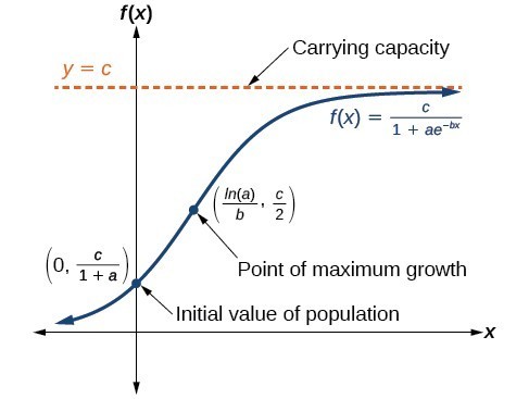
Figure 7

A General Note: Logistic Growth

The logistic growth model is

[latex]f\left(x\right)=\dfrac{c}{1+a{e}^{-bx}}[/latex]

where

• [latex]\frac{c}{1+a}[/latex] is the initial value
• c is the carrying capacity, or limiting value
• b is a constant determined by the rate of growth.

Example 8: Using the Logistic-Growth Model

An influenza epidemic spreads through a population rapidly, at a rate that depends on two factors: The more people who have the flu, the more rapidly it spreads, and also the more uninfected people there are, the more rapidly it spreads. These two factors make the logistic model a good one to study the spread of communicable diseases. And, clearly, there is a maximum value for the number of people infected: the entire population.

For example, at time t = 0 there is one person in a community of 1,000 people who has the flu. So, in that community, at most 1,000 people can have the flu. Researchers find that for this particular strain of the flu, the logistic growth constant is b = 0.6030. Estimate the number of people in this community who will have had this flu after ten days. Predict how many people in this community will have had this flu after a long period of time has passed.

Show Solution

We substitute the given data into the logistic growth model

[latex]f\left(x\right)=\frac{c}{1+a{e}^{-bx}}[/latex]

Because at most 1,000 people, the entire population of the community, can get the flu, we know the limiting value is c = 1000. To find a, we use the formula that the number of cases at time t = 0 is [latex]\frac{c}{1+a}=1[/latex], from which it follows that a = 999. This model predicts that, after ten days, the number of people who have had the flu is [latex]f\left(x\right)=\frac{1000}{1+999{e}^{-0.6030x}}\approx 293.8[/latex]. Because the actual number must be a whole number (a person has either had the flu or not) we round to 294. In the long term, the number of people who will contract the flu is the limiting value, c = 1000.

Analysis of the Solution

Remember that, because we are dealing with a virus, we cannot predict with certainty the number of people infected. The model only approximates the number of people infected and will not give us exact or actual values.

Figure 8 gives a good picture of how this model fits the data.

Try It

Using the model in Example 5, estimate the number of cases of flu on day 15.

Show Solution

895 cases on day 15

Try It

Expressing an Exponential Model in Base e

While powers and logarithms of any base can be used in modeling, the two most common bases are [latex]10[/latex] and [latex]e[/latex]. In science and mathematics, the base e is often preferred. We can use laws of exponents and laws of logarithms to change any base to base e.

How To: Given a model with the form [latex]y=a{b}^{x}[/latex], change it to the form [latex]y={A}_{0}{e}^{kx}[/latex].

1. Rewrite [latex]y=a{b}^{x}[/latex] as [latex]y=a{e}^{\mathrm{ln}\left({b}^{x}\right)}[/latex].
2. Use the power rule of logarithms to rewrite y as [latex]y=a{e}^{x\mathrm{ln}\left(b\right)}=a{e}^{\mathrm{ln}\left(b\right)x}[/latex].
3. Note that [latex]a={A}_{0}[/latex] and [latex]k=\mathrm{ln}\left(b\right)[/latex] in the equation [latex]y={A}_{0}{e}^{kx}[/latex].

Example 9: Changing to base e

Change the function [latex]y=2.5{\left(3.1\right)}^{x}[/latex] so that this same function is written in the form [latex]y={A}_{0}{e}^{kx}[/latex].

Show Solution

The formula is derived as follows

[latex]\begin{align}y&=2.5{\left(3.1\right)}^{x} \\ &=2.5{e}^{\mathrm{ln}\left({3.1}^{x}\right)}&& \text{Insert exponential and its inverse.} \\ &=2.5{e}^{x\mathrm{ln}3.1}&& \text{Laws of logs.} \\ &=2.5{e}^{\left(\mathrm{ln}3.1\right)}{}^{x}&& \text{Commutative law of multiplication} \end{align}[/latex]

Try It

Change the function [latex]y=3{\left(0.5\right)}^{x}[/latex] to one having e as the base.

Show Solution

[latex]y=3{e}^{\left(\mathrm{ln}0.5\right)x}[/latex]

Try It

Key Equations

Half-life formula	If [latex]\text{ }A={A}_{0}{e}^{kt}[/latex], k < 0, the half-life is [latex]t=-\frac{\mathrm{ln}\left(2\right)}{k}[/latex].
Carbon-14 dating	[latex]t=\frac{\mathrm{ln}\left(\frac{A}{{A}_{0}}\right)}{-0.000121}[/latex].[latex]{A}_{0}[/latex] A is the amount of carbon-14 when the plant or animal died t is the amount of carbon-14 remaining today is the age of the fossil in years
Doubling time formula	If [latex]A={A}_{0}{e}^{kt}[/latex], k > 0, the doubling time is [latex]t=\frac{\mathrm{ln}2}{k}[/latex]
Newton’s Law of Cooling	[latex]T\left(t\right)=A{e}^{kt}+{T}_{s}[/latex], where [latex]{T}_{s}[/latex] is the ambient temperature, [latex]A=T\left(0\right)-{T}_{s}[/latex], and k is the continuous rate of cooling.

Key Concepts

• The basic exponential function is [latex]f\left(x\right)=a{b}^{x}[/latex]. If b > 1, we have exponential growth; if 0 < b < 1, we have exponential decay.
• We can also write this formula in terms of continuous growth as [latex]A={A}_{0}{e}^{kx}[/latex], where [latex]{A}_{0}[/latex] is the starting value. If [latex]{A}_{0}[/latex] is positive, then we have exponential growth when k > 0 and exponential decay when k < 0.
• In general, we solve problems involving exponential growth or decay in two steps. First, we set up a model and use the model to find the parameters. Then we use the formula with these parameters to predict growth and decay.
• We can find the age, t, of an organic artifact by measuring the amount, k, of carbon-14 remaining in the artifact and using the formula [latex]t=\frac{\mathrm{ln}\left(k\right)}{-0.000121}[/latex] to solve for t.
• Given a substance’s doubling time or half-time, we can find a function that represents its exponential growth or decay.
• We can use Newton’s Law of Cooling to find how long it will take for a cooling object to reach a desired temperature, or to find what temperature an object will be after a given time.
• We can use logistic growth functions to model real-world situations where the rate of growth changes over time, such as population growth, spread of disease, and spread of rumors.
• We can use real-world data gathered over time to observe trends. Knowledge of linear, exponential, logarithmic, and logistic graphs help us to develop models that best fit our data.
• Any exponential function with the form [latex]y=a{b}^{x}[/latex] can be rewritten as an equivalent exponential function with the form [latex]y={A}_{0}{e}^{kx}[/latex] where [latex]k=\mathrm{ln}b[/latex].

Glossary

carrying capacity

in a logistic model, the limiting value of the output

doubling time

the time it takes for a quantity to double

half-life

the length of time it takes for a substance to exponentially decay to half of its original quantity

logistic growth model

a function of the form [latex]f\left(x\right)=\frac{c}{1+a{e}^{-bx}}[/latex] where [latex]\frac{c}{1+a}[/latex] is the initial value, c is the carrying capacity, or limiting value, and b is a constant determined by the rate of growth

Newton’s Law of Cooling

the scientific formula for temperature as a function of time as an object’s temperature is equalized with the ambient temperature

order of magnitude

the power of ten, when a number is expressed in scientific notation, with one non-zero digit to the left of the decimal

Section 3.5 Homework Exercises

1. With what kind of exponential model would half-life be associated? What role does half-life play in these models?

2. What is carbon dating? Why does it work? Give an example in which carbon dating would be useful.

3. With what kind of exponential model would doubling time be associated? What role does doubling time play in these models?

4. Why use a logistic model instead of an exponential model?

5. The population of a colony of flies fits an exponential growth model. If there are 1000 flies initially and there are 1800 after 1 day, answer the following:
a) What is the exponential growth model where t represents the number of days?
b) What is the size of the colony after 4 days? Round to the nearest whole number.
c) How long is it until there are 30,000 flies? Round to the nearest tenth.

6. The population of a colony of gnats fits an exponential growth model. If there are 500 gnats initially and there are 800 after 1 day, answer the following:
a) What is the exponential growth model where t represents the number of days?
b) What is the size of the colony after 4 days? Round to the nearest whole number.
c) How long is it until there are 90,000 gnats? Round to the nearest tenth.

For the following exercises, use the logistic growth model [latex]f\left(x\right)=\frac{150}{1+8{e}^{-2x}}[/latex].

7. Find and interpret [latex]f\left(0\right)[/latex]. Round to the nearest tenth.

8. Find and interpret [latex]f\left(4\right)[/latex]. Round to the nearest tenth.

9. Find the carrying capacity.

10. Graph the model.

11. Determine whether the data from the table could best be represented as a function that is linear, exponential, or logarithmic. Then write a formula for a model that represents the data.

x f (x)
–2 0.694
–1 0.833
0 1
1 1.2
2 1.44
3 1.728
4 2.074
5 2.488

12. Rewrite [latex]f\left(x\right)=1.68{\left(0.65\right)}^{x}[/latex] as an exponential equation with base e to five significant digits.

For the following exercises, use a graphing calculator and this scenario: the population of a fish farm in t years is modeled by the equation [latex]P\left(t\right)=\frac{1000}{1+9{e}^{-0.6t}}[/latex].

13. Graph the function.

14. What is the initial population of fish?

15. To the nearest tenth, what is the doubling time for the fish population?

16. To the nearest whole number, what will the fish population be after 2 years?

17. To the nearest tenth, how long will it take for the population to reach 900?

18. What is the carrying capacity for the fish population? Justify your answer using the graph of P.

19. A substance has a half-life of 2.045 minutes. If the initial amount of the substance was 132.8 grams, how many half-lives will have passed before the substance decays to 8.3 grams? What is the total time of decay?

20. The formula for an increasing population is given by [latex]P\left(t\right)={P}_{0}{e}^{rt}[/latex] where [latex]{P}_{0}[/latex] is the initial population and r > 0. Derive a general formula for the time t it takes for the population to increase by a factor of M.

21. Recall the formula for calculating the magnitude of an earthquake, [latex]M=\frac{2}{3}\mathrm{log}\left(\frac{S}{{S}_{0}}\right)[/latex]. Show each step for solving this equation algebraically for the seismic moment S.

22. What is the y-intercept of the logistic growth model [latex]y=\frac{c}{1+a{e}^{-rx}}[/latex]? Show the steps for calculation. What does this point tell us about the population?

23. Prove that [latex]{b}^{x}={e}^{x\mathrm{ln}\left(b\right)}[/latex] for positive [latex]b\ne 1[/latex].

For the following exercises, use this scenario: A doctor prescribes 125 milligrams of a therapeutic drug that decays by about 30% each hour.

24. To the nearest hour, what is the half-life of the drug?

25. Write an exponential model representing the amount of the drug remaining in the patient’s system after t hours. Then use the formula to find the amount of the drug that would remain in the patient’s system after 3 hours. Round to the nearest milligram.

26. Using the model found in the previous exercise, find [latex]f\left(10\right)[/latex] and interpret the result. Round to the nearest hundredth.

For the following exercises, use this scenario: A tumor is injected with 0.5 grams of Iodine-125, which has a decay rate of 1.15% per day.

27. To the nearest day, how long will it take for half of the Iodine-125 to decay?

28. Write an exponential model representing the amount of Iodine-125 remaining in the tumor after t days. Then use the formula to find the amount of Iodine-125 that would remain in the tumor after 60 days. Round to the nearest tenth of a gram.

29. A scientist begins with 250 grams of a radioactive substance. After 250 minutes, the sample has decayed to 32 grams. Rounding to five significant digits, write an exponential equation representing this situation. To the nearest minute, what is the half-life of this substance?

30. The half-life of Radium-226 is 1590 years. What is the annual decay rate? Express the decimal result to four significant digits and the percentage to two significant digits.

31. The half-life of Erbium-165 is 10.4 hours. What is the hourly decay rate? Express the decimal result to four significant digits and the percentage to two significant digits.

32. A wooden artifact from an archeological dig contains 60 percent of the carbon-14 that is present in living trees. To the nearest year, about how many years old is the artifact? (The half-life of carbon-14 is 5730 years.)

33. A research student is working with a culture of bacteria that doubles in size every twenty minutes. The initial population count was 1350 bacteria. Rounding to five significant digits, write an exponential equation representing this situation. To the nearest whole number, what is the population size after 3 hours?

For the following exercises, use this scenario: A biologist recorded a count of 360 bacteria present in a culture after 5 minutes and 1000 bacteria present after 20 minutes.

34. To the nearest whole number, what was the initial population in the culture?

35. Rounding to six significant digits, write an exponential equation representing this situation. To the nearest minute, how long did it take the population to double?

36. Plot each set of approximate values of intensity of sounds on a logarithmic scale: Whisper: [latex]{10}^{-10} \frac{W}{{m}^{2}}[/latex], Vacuum: [latex]{10}^{-4}\frac{W}{{m}^{2}}[/latex], Jet: [latex]{10}^{2} \frac{W}{{m}^{2}}[/latex]

37. Recall the formula for calculating the magnitude of an earthquake, [latex]M=\frac{2}{3}\mathrm{log}\left(\frac{S}{{S}_{0}}\right)[/latex]. One earthquake has magnitude 3.9 on the MMS scale. If a second earthquake has 750 times as much energy as the first, find the magnitude of the second quake. Round to the nearest hundredth.

For the following exercises, use this scenario: The equation [latex]N\left(t\right)=\frac{500}{1+49{e}^{-0.7t}}[/latex] models the number of people in a town who have heard a rumor after t days.

38. How many people started the rumor?

39. To the nearest whole number, how many people will have heard the rumor after 3 days?

40. As t increases without bound, what value does N(t) approach? Interpret your answer.

For the following exercise, choose the correct answer choice.

41. A doctor and injects a patient with 13 milligrams of radioactive dye that decays exponentially. After 12 minutes, there are 4.75 milligrams of dye remaining in the patient’s system. Which is an appropriate model for this situation?

A. [latex]f\left(t\right)=13{\left(0.0805\right)}^{t}[/latex]
B. [latex]f\left(t\right)=13{e}^{0.9195t}[/latex]
C. [latex]f\left(t\right)=13{e}^{\left(-0.0839t\right)}[/latex]
D. [latex]f\left(t\right)=\frac{4.75}{1+13{e}^{-0.83925t}}[/latex]