Learning Outcomes
- Identify polynomial functions
- Identify the degree, leading coefficient, and multiplicity of polynomial functions
- Identify end behavior of polynomial functions.
- Identify behavior at each zero
- Graph polynomial functions
- Use the Intermediate Value Theorem.
- Writing a formula for a polynomial function from the graph
Identify polynomial functions
An oil pipeline bursts in the Gulf of Mexico, causing an oil slick in a roughly circular shape. The slick is currently 24 miles in radius, but that radius is increasing by 8 miles each week. We want to write a formula for the area covered by the oil slick by combining two functions. The radius r of the spill depends on the number of weeks w that have passed. This relationship is linear.
We can combine this with the formula for the area A of a circle.
Composing these functions gives a formula for the area in terms of weeks.
Multiplying gives the formula.
This formula is an example of a polynomial function. A polynomial function consists of either zero or the sum of a finite number of non-zero terms, each of which is a product of a number, called the coefficient of the term, and a variable raised to a non-negative integer power.
A General Note: Polynomial Functions
Let n be a non-negative integer. A polynomial function is a function that can be written in the form
[latex]f\left(x\right)={a}_{n}{x}^{n}+\dots+{a}_{2}{x}^{2}+{a}_{1}x+{a}_{0}[/latex]
This is called the general form of a polynomial function. Each [latex]{a}_{i}[/latex] is a coefficient and can be any real number. Each product [latex]{a}_{i}{x}^{i}[/latex] is a term of a polynomial function.
Characteristics of Polynomial Functions
- A polynomial function consists of either zero or the sum of a finite number of non-zero terms
- A polynomial must have whole number exponents [latex](0,1,2,3,...)[/latex]
- A polynomial cannot have negative, fractional, or decimal exponents
- A polynomial must be a smooth continuous curve with no breaks or cusps
Example 1: Identifying Polynomial Functions
Which of the following are polynomial functions?
[latex]\begin{gathered}f\left(x\right)=2{x}^{3}\cdot 3x+4 \\ g\left(x\right)=-x\left({x}^{2}-4\right) \\ h\left(x\right)=5\sqrt{x}+2 \end{gathered}[/latex]
Identify the degree and leading coefficient of polynomial functions
Because of the form of a polynomial function, we can see an infinite variety in the number of terms and the power of the variable. Although the order of the terms in the polynomial function is not important for performing operations, we typically arrange the terms in descending order of power, or in general form. The degree of the polynomial is the highest power of the variable that occurs in the polynomial; it is the power of the first variable if the function is in general form. The leading term is the term containing the highest power of the variable, or the term with the highest degree. The leading coefficient is the coefficient of the leading term.
A General Note: Terminology of Polynomial Functions
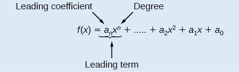
Figure 1
We often rearrange polynomials so that the powers are descending.
When a polynomial is written in this way, we say that it is in general form.
How To: Given a polynomial function, identify the degree and leading coefficient.
- Find the highest power of x to determine the degree function.
- Identify the term containing the highest power of x to find the leading term.
- Identify the coefficient of the leading term.
Example 2: Identifying the Degree and Leading Coefficient of a Polynomial Function
Identify the degree, leading term, and leading coefficient of the following polynomial functions.
[latex]\begin{gathered} f\left(x\right)=3+2{x}^{2}-4{x}^{3} \\ g\left(t\right)=5{t}^{5}-2{t}^{3}+7t\\ h\left(p\right)=6p-{p}^{3}-2\end{gathered}[/latex]
Try It 1
Identify the degree, leading term, and leading coefficient of the polynomial [latex]f\left(x\right)=4{x}^{2}-{x}^{6}+2x - 6[/latex].
Try It 2
Identifying Local Behavior of Polynomial Functions
A turning point is a point at which the function values change from increasing to decreasing or decreasing to increasing.
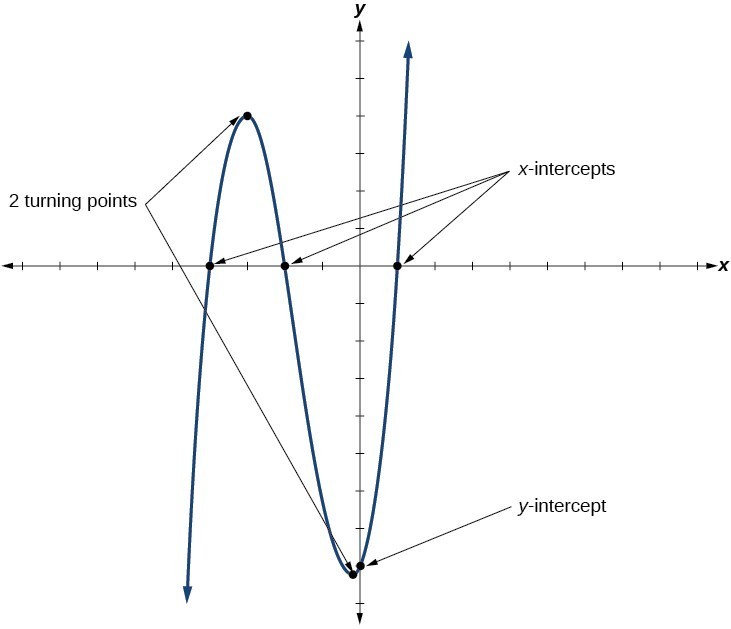
Figure 2
Understand the relationship between degree and turning points
Look at the graph of the polynomial function [latex]f\left(x\right)={x}^{4}-{x}^{3}-4{x}^{2}+4x[/latex] in Figure 3. The graph has three turning points.
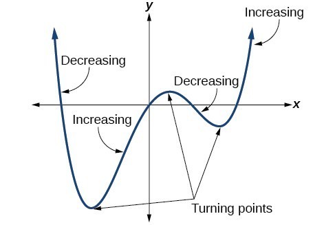
Figure 3
This function f is a 4th degree polynomial function and has 3 turning points. The maximum number of turning points of a polynomial function is always one less than the degree of the function.
A General Note: Interpreting Turning Points
A turning point is a point of the graph where the graph changes from increasing to decreasing (rising to falling) or decreasing to increasing (falling to rising).
A polynomial of degree n will have at most n – 1 turning points.
Example 3: Finding the Maximum Number of Turning Points Using the Degree of a Polynomial Function
Find the maximum number of turning points of each polynomial function.
- [latex]f\left(x\right)=-{x}^{3}+4{x}^{5}-3{x}^{2}++1[/latex]
- [latex]f\left(x\right)=-{\left(x - 1\right)}^{2}\left(1+2{x}^{2}\right)[/latex]

Try It 3
Without graphing the function, determine the maximum number of turning points for [latex]f\left(x\right)=108 - 13{x}^{9}-8{x}^{4}+14{x}^{12}+2{x}^{3}[/latex]
Comparing Smooth and Continuous Graphs
The degree of a polynomial function helps us to determine the number of turning points. A polynomial function of nth degree is the product of n factors, so it will have at most n roots or zeros, or x-intercepts. The graph of the polynomial function of degree n must have at most n – 1 turning points. This means the graph has at most one fewer turning point than the degree of the polynomial or one fewer than the number of factors.
A continuous function has no breaks in its graph: the graph can be drawn without lifting the pen from the paper. A smooth curve is a graph that has no sharp corners. The turning points of a smooth graph must always occur at rounded curves. The graphs of polynomial functions are both continuous and smooth.
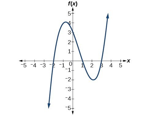
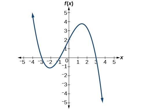
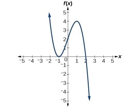
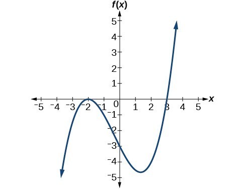
Example 4: Recognizing Polynomial Functions
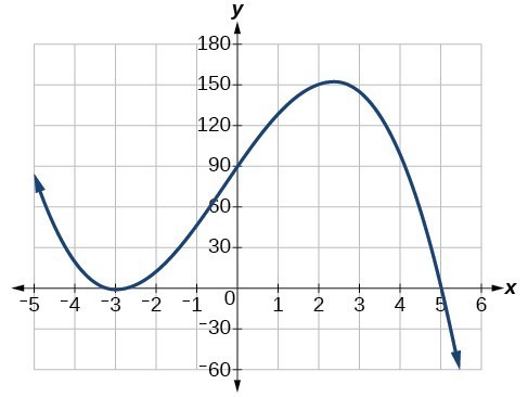
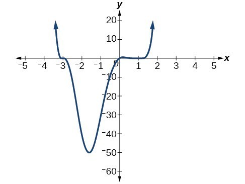
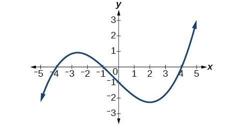
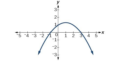
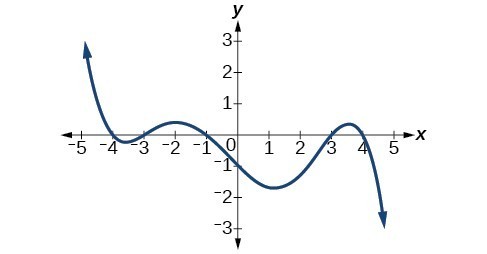
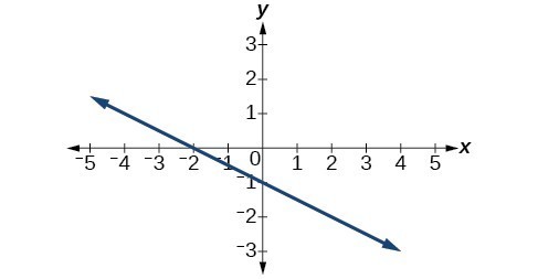
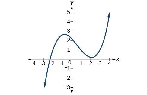
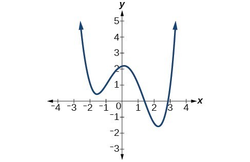
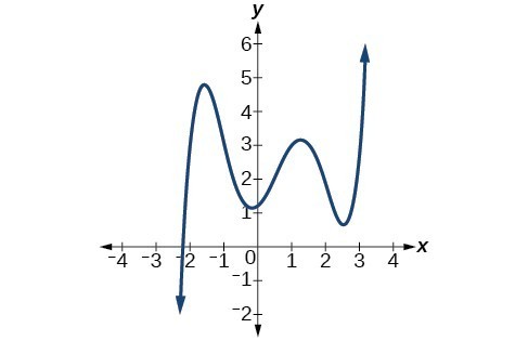
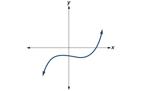
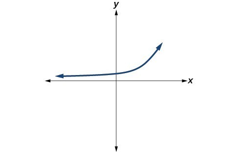
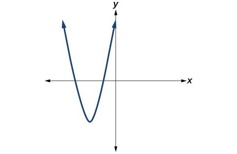
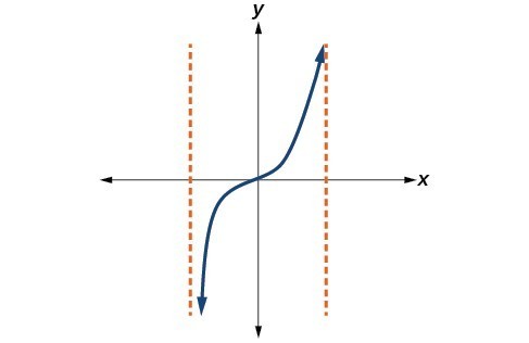
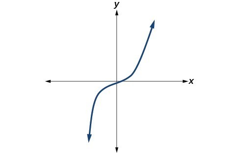
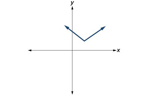
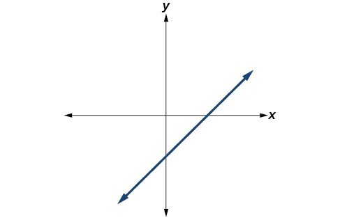
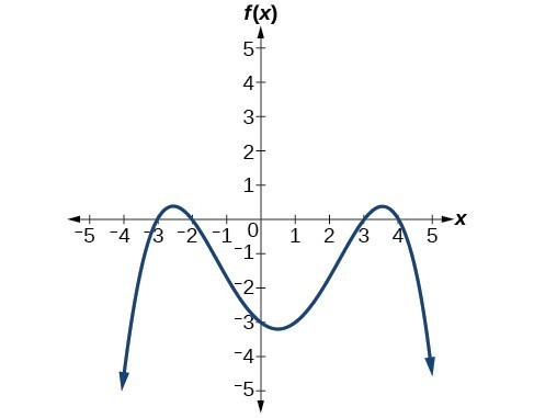
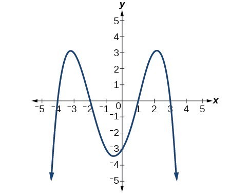
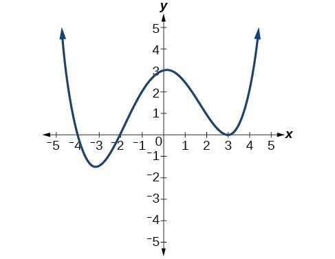
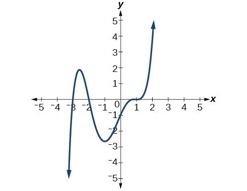
Which of the graphs in Figure 4 represents a degree 3 polynomial function?
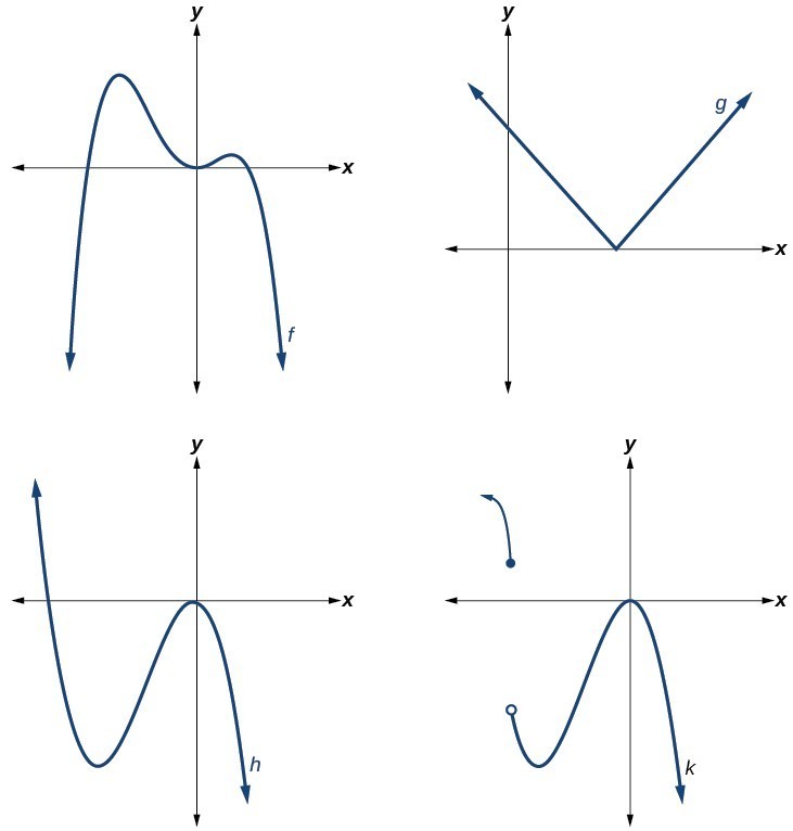
Figure 4
The Factor Theorem
For the polynomial [latex]P(x)[/latex],
- If [latex]r[/latex] is a zero of [latex]P(x)[/latex] then [latex]x-r[/latex] will be a factor of [latex]P(x)[/latex].
- If [latex]x-r[/latex] is a factor of [latex]P(x)[/latex] then [latex]r[/latex] will be a zero of [latex]P(x)[/latex].
Example 5: Form a polynomial from given zeros
Given [latex]f(x)[/latex] has zeros of [latex]-5,0,5[/latex], form a degree three polynomial with integer coefficients.
Example 6: Form a polynomial from given zeros
Given [latex]f(x)[/latex] has zeros of [latex]-3,2[/latex], form a degree three polynomial with integer coefficients.
In the previous example, writing a degree polynomial with zeros of [latex]-3,2[/latex] resulted in two answers: [latex]f(x)=(x+3)^{2}(x-2)[/latex] or [latex]f(x)=(x+3)(x-2)^{2}[/latex]. The exponents on each of the factors are called multiplicities.
Multiplicities are useful because they indicate whether a graph touches or crosses the x-axis.
Identify zeros and their multiplicities
Graphs behave differently at various x-intercepts. Sometimes, the graph will cross over the horizontal axis at an intercept. Other times, the graph will touch the horizontal axis and bounce off.
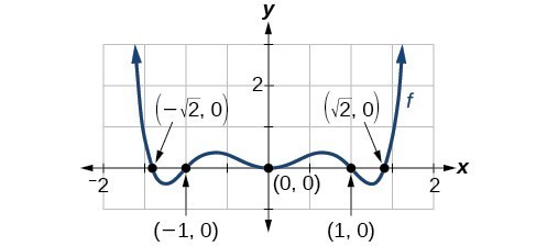
Suppose, for example, we graph the function
Notice in Figure 5 that the behavior of the function at each of the x-intercepts is different.
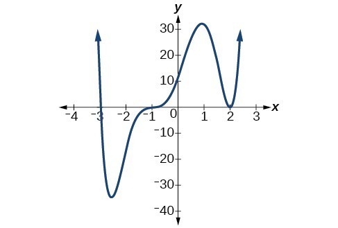
Figure 5. Identifying the behavior of the graph at an x-intercept by examining the multiplicity of the zero.
The x-intercept [latex]x=-3[/latex] is the solution of equation [latex]x+3=0[/latex]. The graph passes directly through the x-intercept at [latex]x=-3[/latex]. The factor is linear (has a degree of 1), so the behavior near the intercept is like that of a line—it passes directly through the intercept. We call this a single zero because the zero corresponds to a single factor of the function.
The x-intercept [latex]x=2[/latex] is the repeated solution of the equation [latex]{\left(x - 2\right)}^{2}=0[/latex]. The graph touches the axis at the intercept and changes direction. The factor is quadratic (degree 2), so the behavior near the intercept is like that of a quadratic—it bounces off of the horizontal axis at the intercept.
The factor is repeated, that is, the factor [latex]\left(x - 2\right)[/latex] appears twice. The number of times a given factor appears in the factored form of the equation of a polynomial is called the multiplicity. The zero associated with this factor, [latex]x=2[/latex], has multiplicity 2 because the factor [latex]\left(x - 2\right)[/latex] occurs twice.
The x-intercept [latex]x=-1[/latex] is the repeated solution of factor [latex]{\left(x+1\right)}^{3}=0[/latex]. The graph passes through the axis at the intercept, but flattens out a bit first. This factor is cubic (degree 3), so the behavior near the intercept is like that of a cubic—with the same S-shape near the intercept as the toolkit function [latex]f\left(x\right)={x}^{3}[/latex]. We call this a triple zero, or a zero with multiplicity 3.
For zeros with even multiplicities, the graphs touch or are tangent to the x-axis. For zeros with odd multiplicities, the graphs cross or intersect the x-axis. See Figure 6 for examples of graphs of polynomial functions with multiplicity 1, 2, and 3.

Figure 6
For higher even powers, such as 4, 6, and 8, the graph will still touch and bounce off of the horizontal axis but, for each increasing even power, the graph will appear flatter as it approaches and leaves the x-axis.
For higher odd powers, such as 5, 7, and 9, the graph will still cross through the horizontal axis, but for each increasing odd power, the graph will appear flatter as it approaches and leaves the x-axis.
A General Note: Graphical Behavior of Polynomials at x-Intercepts
If a polynomial contains a factor of the form [latex]{\left(x-h\right)}^{p}[/latex], the behavior near the x-intercept h is determined by the power p. We say that [latex]x=h[/latex] is a zero of multiplicity p.
The graph of a polynomial function will touch the x-axis at zeros with even multiplicities. The graph will cross the x-axis at zeros with odd multiplicities.
The sum of the multiplicities is the degree of the polynomial function.
How To: Given a graph of a polynomial function of degree n, identify the zeros and their multiplicities.
- If the graph crosses the x-axis and appears almost linear at the intercept, it is a single zero.
- If the graph touches the x-axis and bounces off of the axis, it is a zero with even multiplicity.
- If the graph crosses the x-axis at a zero, it is a zero with odd multiplicity.
- The sum of the multiplicities is n. This includes non-real zeros.
Example 7: Identifying Zeros and Their Multiplicities
Use the graph of the function of degree 6 to identify the zeros of the function and their possible multiplicities.
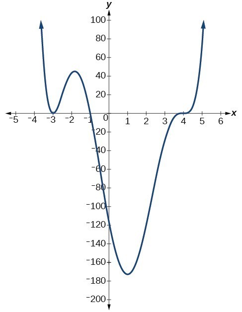
Figure 7
Try It 4
Use the graph of the function of degree 5 to identify the zeros of the function and their multiplicities.
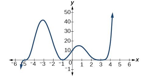
Figure 8
Example 8: Determining zeros and multiplicities of a Polynomial Function
Given the polynomial function [latex]f\left(x\right)=\left(x - 2\right)\left(x+1\right)\left(x - 4\right)[/latex], written in factored form for your convenience, determine the zeros and multiplicities
Use factoring to find zeros of polynomial functions
Find zeros of polynomial functions
Recall that if f is a polynomial function, the values of x for which [latex]f\left(x\right)=0[/latex] are called zeros of f. If the equation of the polynomial function can be factored, we can set each factor equal to zero and solve for the zeros.
We can use this method to find x-intercepts because at the x-intercepts we find the input values when the output value is zero. For general polynomials, this can be a challenging prospect. While quadratics can be solved using the relatively simple quadratic formula, the corresponding formulas for cubic and fourth-degree polynomials are not simple enough to remember, and formulas do not exist for general higher-degree polynomials. Consequently, we will limit ourselves to three cases in this section:
- The polynomial can be factored using known methods: greatest common factor and trinomial factoring.
- The polynomial is given in factored form.
- Technology is used to determine the intercepts.
How To: Given a polynomial function f, find the x-intercepts by factoring.
- Set [latex]f\left(x\right)=0[/latex].
- If the polynomial function is not given in factored form:
- Factor out any common monomial factors.
- Factor any factorable binomials or trinomials.
- Set each factor equal to zero and solve to find the [latex]x\text{-}[/latex] intercepts.
Example 9: Finding the x-Intercepts of a Polynomial Function by Factoring
Find the x-intercepts of [latex]f\left(x\right)={x}^{6}-3{x}^{4}+2{x}^{2}[/latex].
Example 10: Finding the x-Intercepts of a Polynomial Function by Factoring
Find the x-intercepts of [latex]f\left(x\right)={x}^{3}-5{x}^{2}-x+5[/latex].

Example 11: Finding the y– and x-Intercepts of a Polynomial in Factored Form
Find the y– and x-intercepts of [latex]g\left(x\right)={\left(x - 2\right)}^{2}\left(2x+3\right)[/latex].
Example 12: Finding the x-Intercepts of a Polynomial Function Using a Graph
Find the x-intercepts of [latex]h\left(x\right)={x}^{3}+4{x}^{2}+x - 6[/latex].
Try It 5
Find the y– and x-intercepts of the function [latex]f\left(x\right)={x}^{4}-19{x}^{2}+30x[/latex].
Try it 6
Determine behavior at each zero
The behavior at each zero indicates what the graph will look like when it crosses the x-axis. It will resemble a function. Once the behavior at each zero is found, a rough sketch of these behavior equations can be drawn at each zero to aid in graphing the polynomial.
How To: Find the behavior at each zero
- Put the zero into the function for x everywhere except the factor that generated the zero.
- Simplify the expression.
Example 13: Finding the behavior at each zero
Find the behavior at each zero if [latex]f\left(x\right)=x(x-4)^{2}(x+1)^{3}[/latex].
Try It 7
Find the behavior at each zero if [latex]f\left(x\right)=x^{2}(x-2)^{3}(x+3)[/latex].
Determine end behavior
As we have already learned, the behavior of a graph of a polynomial function of the form
will either ultimately rise or fall as x increases without bound and will either rise or fall as x decreases without bound. This is because for very large inputs, say 100 or 1,000, the leading term dominates the size of the output. The same is true for very small inputs, say –100 or –1,000.
Recall that we call this behavior the end behavior of a function. As we pointed out when discussing quadratic equations, when the leading term of a polynomial function, [latex]{a}_{n}{x}^{n}[/latex], is an even power function, as x increases or decreases without bound, [latex]f\left(x\right)[/latex] increases without bound. When the leading term is an odd power function, as x decreases without bound, [latex]f\left(x\right)[/latex] also decreases without bound; as x increases without bound, [latex]f\left(x\right)[/latex] also increases without bound. If the leading term is negative, it will change the direction of the end behavior. The table below summarizes all four cases.
| Even Degree | Odd Degree |
|---|---|
 |
 |
 |
 |
Graph polynomial functions
We can use what we have learned about multiplicities, end behavior, and turning points to sketch graphs of polynomial functions. Let us put this all together and look at the steps required to graph polynomial functions.
How To: Given a polynomial function, sketch the graph.
- Find the zeros and the y-intercept. Plot them. Find the multiplicities.
- Find the behavior at each zero. Make a small sketch of this behavior equation at each zero.
- Determine the end behavior by examining the leading term.
- Use the end behavior and the behavior at each zero to sketch a graph.
- Ensure that the number of turning points does not exceed one less than the degree of the polynomial.
- Optionally, use technology to check the graph.
Example 14: Sketching the Graph of a Polynomial Function
Sketch a graph of [latex]f\left(x\right)=-2{\left(x+3\right)}^{2}\left(x - 5\right)[/latex].

Try It 8
Sketch a graph of [latex]f\left(x\right)=\frac{1}{4}x{\left(x - 1\right)}^{4}{\left(x+3\right)}^{3}[/latex].
Use the Intermediate Value Theorem
In some situations, we may know two points on a graph but not the zeros. If those two points are on opposite sides of the x-axis, we can confirm that there is a zero between them. Consider a polynomial function f whose graph is smooth and continuous. The Intermediate Value Theorem states that for two numbers a and b in the domain of f, if a < b and [latex]f\left(a\right)\ne f\left(b\right)[/latex], then the function f takes on every value between [latex]f\left(a\right)[/latex] and [latex]f\left(b\right)[/latex].
We can apply this theorem to a special case that is useful in graphing polynomial functions. If a point on the graph of a continuous function f at [latex]x=a[/latex] lies above the x-axis and another point at [latex]x=b[/latex] lies below the x-axis, there must exist a third point between [latex]x=a[/latex] and [latex]x=b[/latex] where the graph crosses the x-axis. Call this point [latex]\left(c,\text{ }f\left(c\right)\right)[/latex]. This means that we are assured there is a solution c where [latex]f\left(c\right)=0[/latex].
In other words, the Intermediate Value Theorem tells us that when a polynomial function changes from a negative value to a positive value, the function must cross the x-axis. Figure 18 shows that there is a zero between a and b.
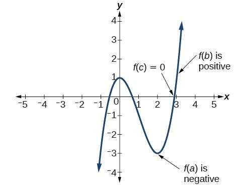
Figure 18. Using the Intermediate Value Theorem to show there exists a zero.
A General Note: Intermediate Value Theorem
Let f be a polynomial function. The Intermediate Value Theorem states that if [latex]f\left(a\right)[/latex] and [latex]f\left(b\right)[/latex] have opposite signs, then there exists at least one value c between a and b for which [latex]f\left(c\right)=0[/latex].
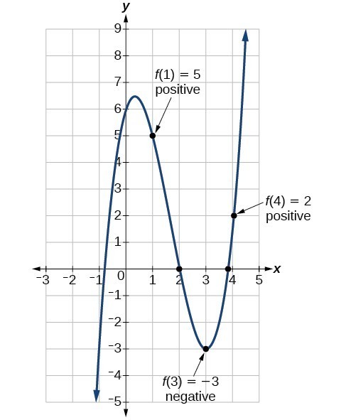
Example 15: Using the Intermediate Value Theorem
Show that the function [latex]f\left(x\right)={x}^{3}-5{x}^{2}+3x+6[/latex] has at least two real zeros between [latex]x=1[/latex] and [latex]x=4[/latex].
Try It 9
Show that the function [latex]f\left(x\right)=7{x}^{5}-9{x}^{4}-{x}^{2}[/latex] has at least one real zero between [latex]x=1[/latex] and [latex]x=2[/latex].
Writing Formulas for Polynomial Functions
Now that we know how to find zeros of polynomial functions, we can use them to write formulas based on graphs. Because a polynomial function written in factored form will have an x-intercept where each factor is equal to zero, we can form a function that will pass through a set of x-intercepts by introducing a corresponding set of factors.
A General Note: Factored Form of Polynomials
If a polynomial of lowest degree p has horizontal intercepts at [latex]x={x}_{1},{x}_{2},\dots ,{x}_{n}[/latex], then the polynomial can be written in the factored form: [latex]f\left(x\right)=a{\left(x-{x}_{1}\right)}^{{p}_{1}}{\left(x-{x}_{2}\right)}^{{p}_{2}}\cdots {\left(x-{x}_{n}\right)}^{{p}_{n}}[/latex] where the powers [latex]{p}_{i}[/latex] on each factor can be determined by the behavior of the graph at the corresponding intercept, and the stretch factor a can be determined given a value of the function other than the x-intercept.
How To: Given a graph of a polynomial function, write a formula for the function.
- Identify the x-intercepts of the graph to find the factors of the polynomial.
- Examine the behavior of the graph at the x-intercepts to determine the multiplicity of each factor.
- Find the polynomial of least degree containing all the factors found in the previous step.
- Use any other point on the graph (the y-intercept may be easiest) to determine the stretch factor.
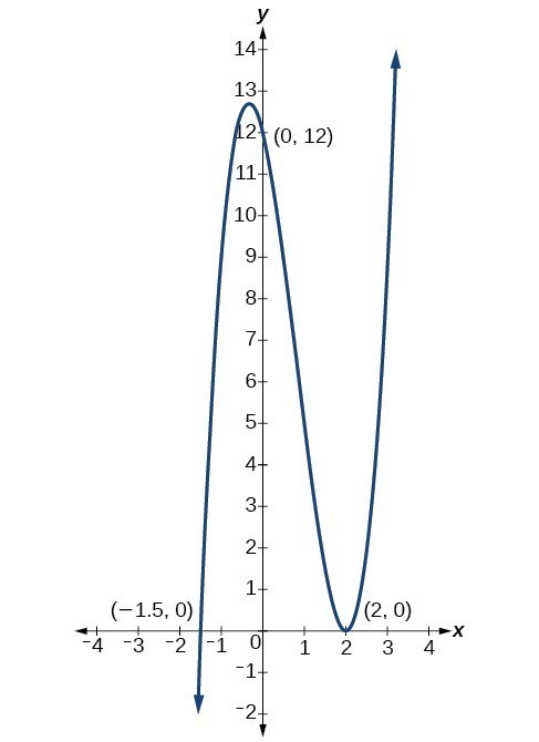
Example 16: Writing a Formula for a Polynomial Function from the Graph
Write a formula for the polynomial function shown in Figure 20.
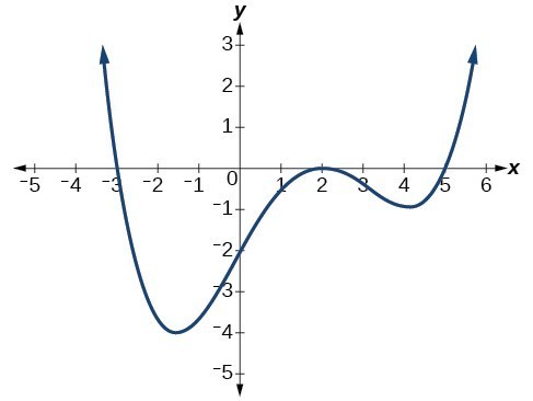
Figure 20
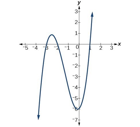
Try It 10
Given the graph in Figure 20, write a formula for the function shown.

Figure 21
Try It 11
Using Local and Global Extrema
With quadratics, we were able to algebraically find the maximum or minimum value of the function by finding the vertex. For general polynomials, finding these turning points is not possible without more advanced techniques from calculus. Even then, finding where extrema occur can still be algebraically challenging. For now, we will estimate the locations of turning points using technology to generate a graph.
Each turning point represents a local minimum or maximum. Sometimes, a turning point is the highest or lowest point on the entire graph. In these cases, we say that the turning point is a global maximum or a global minimum. These are also referred to as the absolute maximum and absolute minimum values of the function.
Local and Global Extrema
A local maximum or local minimum at x = a (sometimes called the relative maximum or minimum, respectively) is the output at the highest or lowest point on the graph in an open interval around x = a. If a function has a local maximum at a, then [latex]f\left(a\right)\ge f\left(x\right)[/latex] for all x in an open interval around x = a. If a function has a local minimum at a, then [latex]f\left(a\right)\le f\left(x\right)[/latex] for all x in an open interval around x = a.
A global maximum or global minimum is the output at the highest or lowest point of the function. If a function has a global maximum at a, then [latex]f\left(a\right)\ge f\left(x\right)[/latex] for all x. If a function has a global minimum at a, then [latex]f\left(a\right)\le f\left(x\right)[/latex] for all x.
We can see the difference between local and global extrema in Figure 21.
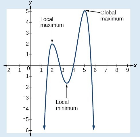
Figure 22
Q & A
Do all polynomial functions have a global minimum or maximum?
No. Only polynomial functions of even degree have a global minimum or maximum. For example, [latex]f\left(x\right)=x[/latex] has neither a global maximum nor a global minimum.
Key Equations
| general form of a polynomial function | [latex]f\left(x\right)={a}_{n}{x}^{n}+\dots+{a}_{2}{x}^{2}+{a}_{1}x+{a}_{0}[/latex] |
Key Concepts
- A polynomial function is the sum of terms, each of which consists of a transformed power function with positive whole number power.
- The degree of a polynomial function is the highest power of the variable that occurs in a polynomial. The term containing the highest power of the variable is called the leading term. The coefficient of the leading term is called the leading coefficient.
- A polynomial of degree n will have at most n x-intercepts and at most n – 1 turning points.
- The graph of a polynomial function changes direction at its turning points.
- Polynomial functions of degree 2 or more are smooth, continuous functions.
- To find the zeros of a polynomial function, if it can be factored, factor the function and set each factor equal to zero.
- Another way to find the x-intercepts of a polynomial function is to graph the function and identify the points at which the graph crosses the x-axis.
- The multiplicity of a zero determines how the graph behaves at the x-intercepts, in addition to the behavior equations at each zero.
- The graph of a polynomial will cross the horizontal axis at a zero with odd multiplicity.
- The graph of a polynomial will touch the horizontal axis at a zero with even multiplicity.
- The end behavior of a polynomial function depends on the leading term.
- To graph polynomial functions, find the zeros and their multiplicities, determine the end behavior, and ensure that the final graph has at most n – 1 turning points.
- Graphing a polynomial function helps to estimate local and global extremas.
- The Intermediate Value Theorem tells us that if [latex]f\left(a\right) \text{and} f\left(b\right)[/latex] have opposite signs, then there exists at least one value c between a and b for which [latex]f\left(c\right)=0[/latex].
Glossary
- coefficient
- a nonzero real number multiplied by a variable raised to an exponent
- continuous function
- a function whose graph can be drawn without lifting the pen from the paper because there are no breaks in the graph
- degree
- the highest power of the variable that occurs in a polynomial
- end behavior
- the behavior of the graph of a function as the input decreases without bound and increases without bound
- global maximum
- highest turning point on a graph; [latex]f\left(a\right)[/latex] where [latex]f\left(a\right)\ge f\left(x\right)[/latex] for all x.
- global minimum
- lowest turning point on a graph; [latex]f\left(a\right)[/latex] where [latex]f\left(a\right)\le f\left(x\right)[/latex]
for all x.
- Intermediate Value Theorem
- for two numbers a and b in the domain of f, if [latex]a
- leading coefficient
- the coefficient of the leading term
- leading term
- the term containing the highest power of the variable
- multiplicity
- the number of times a given factor appears in the factored form of the equation of a polynomial; if a polynomial contains a factor of the form [latex]{\left(x-h\right)}^{p}[/latex], [latex]x=h[/latex] is a zero of multiplicity p.
- polynomial function
- a function that consists of either zero or the sum of a finite number of non-zero terms, each of which is a product of a number, called the coefficient of the term, and a variable raised to a non-negative integer power.
- term of a polynomial function
- any [latex]{a}_{i}{x}^{i}[/latex] of a polynomial function in the form [latex]f\left(x\right)={a}_{n}{x}^{n}+\dots+{a}_{2}{x}^{2}+{a}_{1}x+{a}_{0}[/latex]
- turning point
- the location at which the graph of a function changes direction
Section 2.4 Homework Exercises
1. What is the difference between an x-intercept and a zero of a polynomial function [latex]y[/latex]?
2. If a polynomial function is in factored form, what would be a good first step in order to determine the degree of the function?
3. What is the relationship between the degree of a polynomial function and the maximum number of turning points in its graph?
4. Explain how the Intermediate Value Theorem can assist us in finding a zero of a function.
5. Explain how the factored form of the polynomial helps us in graphing it.
6. If the graph of a polynomial just touches the x-axis and then changes direction, what can we conclude about the factored form of the polynomial?
For the following exercises, determine whether the function is polynomial function. If it is a polynomial function, indicate the degree and [latex]a_{n}[/latex] (leading coefficient).
7. [latex]\text{ }f\left(x\right)=6{x}^{5}[/latex]
8. [latex]\text{ }f\left(x\right)={\left({x}^{2}\right)}^{3}[/latex]
9. [latex]\text{ }f\left(x\right)=\frac{{x}^{2}}{{x}^{2}-1}[/latex]
10. [latex]\text{ }f\left(x\right)=x-{x}^{4}[/latex]
11. [latex]\text{ }f\left(x\right)=2x\left(x+2\right){\left(x - 1\right)}^{2}[/latex]
12. [latex]\text{ }f\left(x\right)={3}^{x+1}[/latex]
13. [latex]\text{ }f\left(x\right)=5\sqrt(x)+2x^{4}[/latex]
14. [latex]\text{ }f\left(x\right)=4x^{2}-\dfrac{3}{x^{3}}[/latex]
For the following exercises, find the intercepts of the functions.
15. [latex]f\left(t\right)=2\left(t - 1\right)\left(t+2\right)\left(t - 3\right)[/latex]
16. [latex]g\left(n\right)=-2\left(3n - 1\right)\left(2n+1\right)[/latex]
17. [latex]f\left(x\right)=-4(x+2)(x-2)[/latex]
18. [latex]f\left(x\right)=\left(x+3\right)\left(4{x}^{2}-1\right)[/latex]
19. [latex]f\left(x\right)=x\left({x}^{2}-2x - 8\right)[/latex]
For the following exercises, determine the least possible degree of the polynomial function shown.
20.
21.
22.
23.
24.
25.
26.
For the following exercises, determine whether the graph of the function provided is a graph of a polynomial function. If so, determine the number of turning points and the least possible degree for the function.
27.
28.
29.
30.
31.
32.
33.
For the following exercises, find the zeros, multiplicity, and the behavior at each zero.
30. [latex]f\left(x\right)={\left(x+2\right)}^{3}{\left(x - 3\right)}^{2}[/latex]
31. [latex]f\left(x\right)={x}^{2}{\left(2x+3\right)}^{3}{\left(x - 4\right)}^{2}[/latex]
32. [latex]f\left(x\right)={x}^{3}{\left(x - 1\right)}^{3}\left(x+2\right)[/latex]
33. [latex]f\left(x\right)={x}^{2}\left({x}^{2}+4x+4\right)[/latex]
34. [latex]f\left(x\right)={\left(2x+1\right)}^{3}\left(9{x}^{2}-6x+1\right)[/latex]
35. [latex]f\left(x\right)={\left(3x+2\right)}^{3}\left({x}^{2}-10x+25\right)[/latex]
36. [latex]f\left(x\right)=x\left(4{x}^{2}-12x+9\right)\left({x}^{2}+8x+16\right)[/latex]
37. [latex]f\left(x\right)={x}^{6}-{x}^{5}-2{x}^{4}[/latex]
38. [latex]f\left(x\right)=3{x}^{4}+6{x}^{3}+3{x}^{2}[/latex]
39. [latex]f\left(x\right)=4{x}^{5}-12{x}^{4}+9{x}^{3}[/latex]
40. [latex]f\left(x\right)=2{x}^{4}\left({x}^{3}-4{x}^{2}+4x\right)[/latex]
41. [latex]f\left(x\right)=4{x}^{4}\left(9{x}^{4}-12{x}^{3}+4{x}^{2}\right)[/latex]
For the following exercises, find the zeros, y-intercept, multiplicity, behavior at each zero, and end behavior. Use these to graph each function.
42. [latex]f\left(x\right)={\left(x+3\right)}^{2}\left(x - 2\right)[/latex]
43. [latex]g\left(x\right)=\left(x+4\right){\left(x - 1\right)}^{2}[/latex]
44. [latex]h\left(x\right)={\left(x - 1\right)}^{3}{\left(x+3\right)}^{2}[/latex]
45. [latex]k\left(x\right)={\left(x - 3\right)}^{3}{\left(x - 2\right)}^{2}[/latex]
46. [latex]m\left(x\right)=-2x\left(x - 1\right)\left(x+3\right)[/latex]
47. [latex]n\left(x\right)=-3x\left(x+2\right)\left(x - 4\right)[/latex]
48. [latex]f\left(x\right)=x^{4}+3x[/latex]
49. [latex]f\left(x\right)=x^{4}-2x[/latex]
For the following exercises, use the information about the graph of a polynomial function to determine the function. Assume the leading coefficient is 1 or –1. There may be more than one correct answer.
50. The y-intercept is [latex]\left(0,-6\right)[/latex]. The x-intercepts are [latex]\left(-3,0\right),\left(2,0\right)[/latex]. Degree is 2.
End behavior: [latex]\text{as }x\to -\infty ,f\left(x\right)\to \infty ,\text{ as }x\to \infty ,f\left(x\right)\to \infty[/latex].
51. The y-intercept is [latex]\left(0,-4\right)[/latex]. The x-intercepts are [latex]\left(-2,0\right),\left(2,0\right)[/latex]. Degree is 2.
End behavior: [latex]\text{as }x\to -\infty ,f\left(x\right)\to \infty ,\text{ as }x\to \infty ,f\left(x\right)\to \infty[/latex].
52. The y-intercept is [latex]\left(0,9\right)[/latex]. The x-intercepts are [latex]\left(-3,0\right),\left(3,0\right)[/latex]. Degree is 2.
End behavior: [latex]\text{as }x\to -\infty ,f\left(x\right)\to -\infty ,\text{ as }x\to \infty ,f\left(x\right)\to -\infty[/latex].
53. The y-intercept is [latex]\left(0,0\right)[/latex]. The x-intercepts are [latex]\left(0,0\right),\left(2,0\right)[/latex]. Degree is 3.
End behavior: [latex]\text{as }x\to -\infty ,f\left(x\right)\to -\infty ,\text{ as }x\to \infty ,f\left(x\right)\to \infty[/latex].
54. The y-intercept is [latex]\left(0,1\right)[/latex]. The x-intercept is [latex]\left(1,0\right)[/latex]. Degree is 3.
End behavior: [latex]\text{as }x\to -\infty ,f\left(x\right)\to \infty ,\text{ as }x\to \infty ,f\left(x\right)\to -\infty[/latex].
55. The y-intercept is [latex]\left(0,1\right)[/latex]. There is no x-intercept. Degree is 4.
End behavior: [latex]\text{as }x\to -\infty ,f\left(x\right)\to \infty ,\text{ as }x\to \infty ,f\left(x\right)\to \infty[/latex].
For the following exercises, use the graphs to write the formula for a polynomial function of least degree.
56.
57.
58.
59.
60.
61.
62.
63.
For the following exercises, use the Intermediate Value Theorem to confirm that the given polynomial has at least one zero within the given interval.
64. [latex]f\left(x\right)={x}^{3}-9x[/latex], between [latex]x=-4[/latex] and [latex]x=-2[/latex].
65. [latex]f\left(x\right)={x}^{3}-9x[/latex], between [latex]x=2[/latex] and [latex]x=4[/latex].
66. [latex]f\left(x\right)={x}^{5}-2x[/latex], between [latex]x=1[/latex] and [latex]x=2[/latex].
67. [latex]f\left(x\right)=-{x}^{4}+4[/latex], between [latex]x=1[/latex] and [latex]x=3[/latex].
68. [latex]f\left(x\right)=-2{x}^{3}-x[/latex], between [latex]x=-1[/latex] and [latex]x=1[/latex].
69. [latex]f\left(x\right)={x}^{3}-100x+2[/latex], between [latex]x=0.01[/latex] and [latex]x=0.1[/latex]