Representing a Linear Function in Word Form

Let’s begin by describing the linear function in words. For the train problem we just considered, the following word sentence may be used to describe the function relationship.

• The train’s distance from the station is a function of the time during which the train moves at a constant speed plus its original distance from the station when it began moving at constant speed.

The speed is the rate of change. Recall that a rate of change is a measure of how quickly the dependent variable changes with respect to the independent variable. The rate of change for this example is constant, which means that it is the same for each input value. As the time (input) increases by 1 second, the corresponding distance (output) increases by 83 meters. The train began moving at this constant speed at a distance of 250 meters from the station.

Representing a Linear Function in Function Notation

Another approach to representing linear functions is by using function notation. One example of function notation is an equation written in the form known as the slope-intercept form of a line, where [latex]x[/latex] is the input value, [latex]m[/latex] is the rate of change, and [latex]b[/latex] is the initial value of the dependent variable.

In the example of the train, we might use the notation [latex]D\left(t\right)[/latex] in which the total distance [latex]D[/latex]
is a function of the time [latex]t[/latex]. The rate, [latex]m[/latex], is 83 meters per second. The initial value of the dependent variable [latex]b[/latex] is the original distance from the station, 250 meters. We can write a generalized equation to represent the motion of the train.

Representing a Linear Function in Tabular Form

A third method of representing a linear function is through the use of a table. The relationship between the distance from the station and the time is represented in the table in Figure 1. From the table, we can see that the distance changes by 83 meters for every 1 second increase in time.

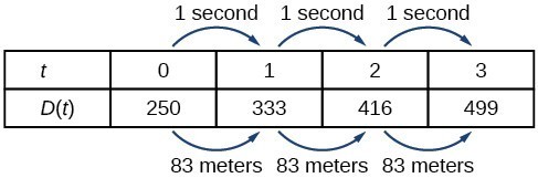
Figure 1. Tabular representation of the function D showing selected input and output values

Representing a Linear Function in Graphical Form

Another way to represent linear functions is visually, using a graph. We can use the function relationship from above, [latex]D(t)=83t+250[/latex], to draw a graph, represented in the graph in Figure 2. Notice the graph is a line. When we plot a linear function, the graph is always a line.

The rate of change, which is constant, determines the slant, or slope of the line. The point at which the input value is zero is the vertical intercept, or y-intercept, of the line. We can see from the graph that the y-intercept in the train example we just saw is [latex]\left(0,250\right)[/latex] and represents the distance of the train from the station when it began moving at a constant speed.

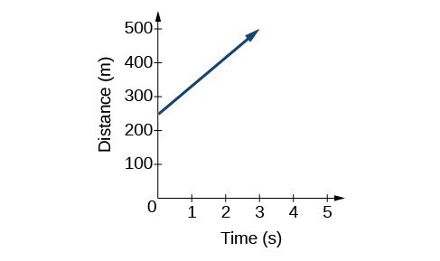
Figure 2. The graph of [latex]D(t)=83t+250[/latex]. Graphs of linear functions are lines because the rate of change is constant.

Notice that the graph of the train example is restricted, but this is not always the case. Consider the graph of the line [latex]f(x)=2{x}_{}+1[/latex]. Ask yourself what numbers can be input to the function, that is, what is the domain of the function? The domain is comprised of all real numbers because any number may be doubled, and then have one added to the product.

Example 1: Using a Linear Function to Find the Pressure on a Diver

The pressure, [latex]P[/latex], in pounds per square inch (PSI) on the diver in Figure 3 depends upon her depth below the water surface, [latex]d[/latex], in feet. This relationship may be modeled by the equation, [latex]P(d)=0.434d+14.696[/latex]. Restate this function in words.

Figure 3. (credit: Ilse Reijs and Jan-Noud Hutten)

Show Solution

To restate the function in words, we need to describe each part of the equation. The pressure as a function of depth equals four hundred thirty-four thousandths times depth plus fourteen and six hundred ninety-six thousandths.

Analysis of the Solution

The initial value, 14.696, is the pressure in PSI on the diver at a depth of 0 feet, which is the surface of the water. The rate of change, or slope, is 0.434 PSI per foot. This tells us that the pressure on the diver increases 0.434 PSI for each foot her depth increases.

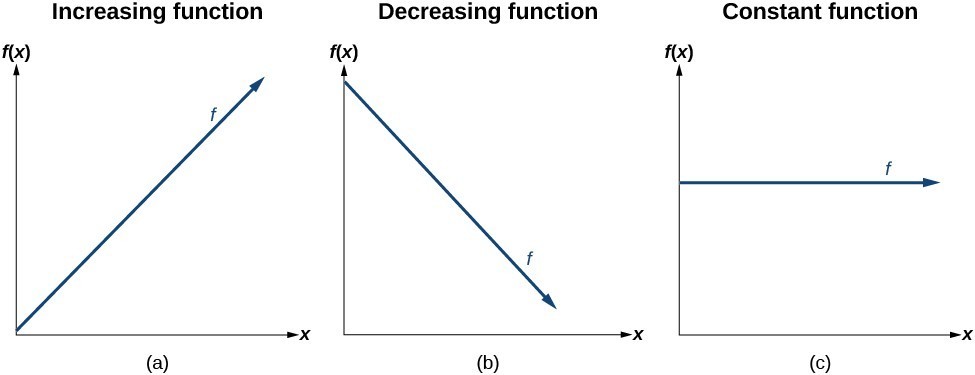
Figure 4

The linear functions we used in the two previous examples increased over time, but not every linear function does. A linear function may be increasing, decreasing, or constant.

For an increasing function, as with the train example,

the output values increase as the input values increase.

The graph of an increasing function has a positive slope. A line with a positive slope slants upward from left to right as in (a).

For a decreasing function, the slope is negative.

The output values decrease as the input values increase.

A line with a negative slope slants downward from left to right as in (b). If the function is constant, the output values are the same for all input values so the slope is zero. A line with a slope of zero is horizontal as in (c).

Calculating and Interpreting Slope

In the examples we have seen so far, we have had the slope provided for us. However, we often need to calculate the slope given input and output values. Given two values for the input, [latex]{x}_{1}[/latex] and [latex]{x}_{2}[/latex], and two corresponding values for the output, [latex]{y}_{1}[/latex] and [latex]{y}_{2}[/latex] —which can be represented by a set of points, [latex]\left({x}_{1}\text{, }{y}_{1}\right)[/latex] and [latex]\left({x}_{2}\text{, }{y}_{2}\right)[/latex]—we can calculate the slope [latex]m[/latex], as follows

where [latex]\Delta y[/latex] is the vertical displacement and [latex]\Delta x[/latex] is the horizontal displacement. Note in function notation two corresponding values for the output [latex]{y}_{1}[/latex] and [latex]{y}_{2}[/latex] for the function [latex]f[/latex], [latex]{y}_{1}=f\left({x}_{1}\right)[/latex] and [latex]{y}_{2}=f\left({x}_{2}\right)[/latex], so we could equivalently write

The graph in Figure 5 indicates how the slope of the line between the points, [latex]\left({x}_{1,}{y}_{1}\right)[/latex]
and [latex]\left({x}_{2,}{y}_{2}\right)[/latex], is calculated. Recall that the slope measures steepness. The greater the absolute value of the slope, the steeper the line is.

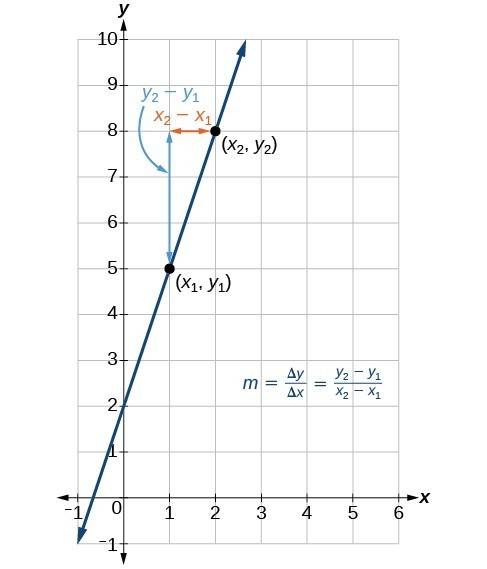
Figure 5

The slope of a function is calculated by the change in [latex]y[/latex] divided by the change in [latex]x[/latex]. It does not matter which coordinate is used as the [latex]\left({x}_{2}\text{,}{y}_{2}\right)[/latex] and which is the [latex]\left({x}_{1}\text{,}{y}_{1}\right)[/latex], as long as each calculation is started with the elements from the same coordinate pair.

Writing the Point-Slope Form of a Linear Equation

Up until now, we have been using the slope-intercept form of a linear equation to describe linear functions. Here, we will learn another way to write a linear function, the point-slope form.

The point-slope form is derived from the slope formula.

Keep in mind that the slope-intercept form and the point-slope form can be used to describe the same function. We can move from one form to another using basic algebra. For example, suppose we are given an equation in point-slope form, [latex]y - 4=-\frac{1}{2}\left(x - 6\right)[/latex] . We can convert it to the slope-intercept form as shown.

Therefore, the same line can be described in slope-intercept form as [latex]y=-\frac{1}{2}x+7[/latex].

Writing the Equation of a Line Using a Point and the Slope

The point-slope form is particularly useful if we know one point and the slope of a line. Suppose, for example, we are told that a line has a slope of 2 and passes through the point [latex]\left(4,1\right)[/latex]. We know that [latex]m=2[/latex] and that [latex]{x}_{1}=4[/latex] and [latex]{y}_{1}=1[/latex]. We can substitute these values into the general point-slope equation.

[latex]\begin{gathered}y-{y}_{1}=m\left(x-{x}_{1}\right)\\ y - 1=2\left(x - 4\right)\end{gathered}[/latex]

[latex][/latex]

If we wanted to then rewrite the equation in slope-intercept form, we apply algebraic techniques.

[latex]\begin{align}&y - 1=2\left(x - 4\right) \\ &y - 1=2x - 8 && \text{Distribute the }2 \\ &y=2x - 7 && \text{Add 1 to each side} \end{align}[/latex]

[latex][/latex]

Both equations, [latex]y - 1=2\left(x - 4\right)[/latex] and [latex]y=2x - 7[/latex], describe the same line. See Figure 6.

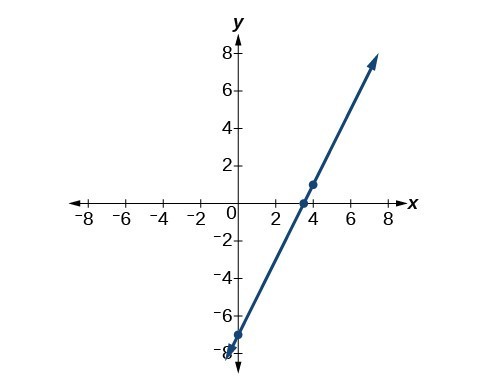
Figure 6

Example 5: Writing Linear Equations Using a Point and the Slope

Write the point-slope form of an equation of a line with a slope of 3 that passes through the point [latex]\left(6,-1\right)[/latex]. Then rewrite it in the slope-intercept form.

Show Solution

Let’s figure out what we know from the given information. The slope is 3, so m = 3. We also know one point, so we know [latex]{x}_{1}=6[/latex] and [latex]{y}_{1}=-1[/latex]. Now we can substitute these values into the general point-slope equation.

[latex]\begin{align}&y-{y}_{1}=m\left(x-{x}_{1}\right) \\ &y-\left(-1\right)=3\left(x - 6\right) && \text{Substitute known values} \\ &y+1=3\left(x - 6\right) && \text{Distribute }-1\text{ to find point-slope form} \end{align}[/latex]

Then we use algebra to find the slope-intercept form.

[latex]\begin{align}&y+1=3\left(x - 6\right) \\ &y+1=3x - 18 && \text{Distribute 3} \\ &y=3x - 19 && \text{Simplify to slope-intercept form} \end{align}[/latex]

Try It

Write the point-slope form of an equation of a line with a slope of –2 that passes through the point [latex]\left(-2,\text{ }2\right)[/latex]. Then rewrite it in the slope-intercept form.

Show Solution

[latex]y - 2=-2\left(x+2\right)[/latex]; [latex]y=-2x - 2[/latex]

Try It

Writing the Equation of a Line Using Two Points

The point-slope form of an equation is also useful if we know any two points through which a line passes. Suppose, for example, we know that a line passes through the points [latex]\left(0,\text{ }1\right)[/latex] and [latex]\left(3,\text{ }2\right)[/latex]. We can use the coordinates of the two points to find the slope.

[latex]\begin{align}{m}&=\frac{{y}_{2}-{y}_{1}}{{x}_{2}-{x}_{1}}\\ &=\frac{2 - 1}{3 - 0} \\ &=\frac{1}{3} \end{align}[/latex]

[latex][/latex]

Now we can use the slope we found and the coordinates of one of the points to find the equation for the line. Let use (0, 1) for our point.

[latex]\begin{align}y-{y}_{1}&=m\left(x-{x}_{1}\right)\\ y - 1&=\frac{1}{3}\left(x - 0\right)\end{align}[/latex]

[latex][/latex]

As before, we can use algebra to rewrite the equation in the slope-intercept form.

[latex]\begin{align}&y - 1=\frac{1}{3}\left(x - 0\right) \\ &y - 1=\frac{1}{3}x && \text{Distribute the }\frac{1}{3} \\ &y=\frac{1}{3}x+1 && \text{Add 1 to each side} \end{align}[/latex]

[latex][/latex]

Both equations describe the line shown in Figure 7.

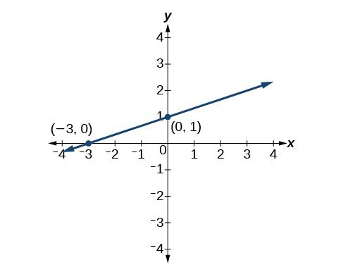
Figure 7

Example 6: Writing Linear Equations Using Two Points

Write the point-slope form of an equation of a line that passes through the points (5, 1) and (8, 7). Then rewrite it in the slope-intercept form.

Show Solution

Let’s begin by finding the slope.

[latex]\begin{align}{m}&=\frac{{y}_{2}-{y}_{1}}{{x}_{2}-{x}_{1}} \\ &=\frac{7 - 1}{8 - 5} \\ &=\frac{6}{3} \\ &=2 \end{align}[/latex]

So [latex]m=2[/latex]. Next, we substitute the slope and the coordinates for one of the points into the general point-slope equation. We can choose either point, but we will use [latex]\left(5,1\right)[/latex].

[latex]\begin{align}y-{y}_{1}&=m\left(x-{x}_{1}\right)\\ y - 1&=2\left(x - 5\right)\end{align}[/latex]

The point-slope equation of the line is [latex]{y}_{2}-1=2\left({x}_{2}-5\right)[/latex]. To rewrite the equation in slope-intercept form, we use algebra.

[latex]\begin{gathered}y - 1=2\left(x - 5\right) \\ y - 1=2x - 10 \\ y=2x - 9 \end{gathered}[/latex]

The slope-intercept equation of the line is [latex]y=2x - 9[/latex].

Try It

Write the point-slope form of an equation of a line that passes through the points [latex]\left(-1,3\right) [/latex] and [latex]\left(0,0\right)[/latex]. Then rewrite it in the slope-intercept form.

Show Solution

[latex]y - 0=-3\left(x - 0\right)[/latex] ; [latex]y=-3x[/latex]

Writing and Interpreting an Equation for a Linear Function

Now that we have written equations for linear functions in both the slope-intercept form and the point-slope form, we can choose which method to use based on the information we are given. That information may be provided in the form of a graph, a point and a slope, two points, and so on. Look at the graph of the function f in Figure 8.

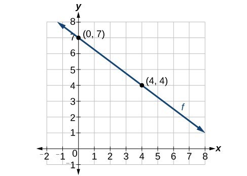
Figure 8

We are not given the slope of the line, but we can choose any two points on the line to find the slope. Let’s choose (0, 7) and (4, 4). We can use these points to calculate the slope.

[latex]\begin{align} m&=\frac{{y}_{2}-{y}_{1}}{{x}_{2}-{x}_{1}} \\ &=\frac{4 - 7}{4 - 0} \\ &=-\frac{3}{4} \end{align}[/latex]
[latex][/latex]

Now we can substitute the slope and the coordinates of one of the points into the point-slope form.

[latex]\begin{gathered}y-{y}_{1}=m\left(x-{x}_{1}\right) \\ y - 4=-\frac{3}{4}\left(x - 4\right) \end{gathered}[/latex]
[latex][/latex]

If we want to rewrite the equation in the slope-intercept form, we would find

[latex]\begin{gathered}y - 4=-\frac{3}{4}\left(x - 4\right)\hfill \\ y - 4=-\frac{3}{4}x+3\hfill \\ \text{ }y=-\frac{3}{4}x+7\hfill \end{gathered}[/latex]

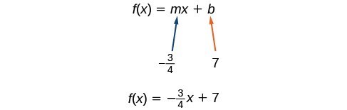
Figure 9

If we wanted to find the slope-intercept form without first writing the point-slope form, we could have recognized that the line crosses the y-axis when the output value is 7. Therefore, b = 7. We now have the initial value b and the slope m so we can substitute m and b into the slope-intercept form of a line.

So the function is [latex]f(xt)=-\frac{3}{4}x+7[/latex], and the linear equation would be [latex]y=-\frac{3}{4}x+7[/latex].

How To: Given the graph of a linear function, write an equation to represent the function.

1. Identify two points on the line.
2. Use the two points to calculate the slope.
3. Determine where the line crosses the y-axis to identify the y-intercept by visual inspection.
4. Substitute the slope and y-intercept into the slope-intercept form of a line equation.

Example 7: Writing an Equation for a Linear Function

Write an equation for a linear function given a graph of f shown in Figure 10.

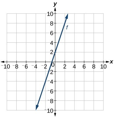
Figure 10

Show Solution

Identify two points on the line, such as (0, 2) and (–2, –4). Use the points to calculate the slope.

[latex]\begin{align} m&=\frac{{y}_{2}-{y}_{1}}{{x}_{2}-{x}_{1}} \\ &=\frac{-4 - 2}{-2 - 0} \\ &=\frac{-6}{-2} \\ &=3 \end{align}[/latex]

Substitute the slope and the coordinates of one of the points into the point-slope form.

[latex]\begin{gathered}y-{y}_{1}=m\left(x-{x}_{1}\right)\\ y-\left(-4\right)=3\left(x-\left(-2\right)\right)\\ y+4=3\left(x+2\right)\end{gathered}[/latex]

We can use algebra to rewrite the equation in the slope-intercept form.

[latex]\begin{gathered}y+4=3\left(x+2\right) \\ y+4=3x+6 \\ y=3x+2 \end{gathered}[/latex]

Analysis of the Solution

This makes sense because we can see from Figure 11 that the line crosses the y-axis at the point (0, 2), which is the y-intercept, so b = 2.

Figure 11

Example 8: Writing an Equation for a Linear Function Given Two Points

If f is a linear function, with [latex]f\left(3\right)=-2[/latex] , and [latex]f\left(8\right)=1[/latex], find an equation for the function in slope-intercept form.

Show Solution

We can write the given points using coordinates.

[latex]\begin{align}&f\left(3\right)=-2\to \left(3,-2\right) \\ &f\left(8\right)=1\to \left(8,1\right) \end{align}[/latex]

We can then use the points to calculate the slope.

[latex]\begin{align} m=&\frac{{y}_{2}-{y}_{1}}{{x}_{2}-{x}_{1}} \\ &=\frac{1-\left(-2\right)}{8 - 3} \\ &=\frac{3}{5} \end{align}[/latex]

Substitute the slope and the coordinates of one of the points into the point-slope form.

[latex]\begin{gathered}y-{y}_{1}=m\left(x-{x}_{1}\right) \\ y-\left(-2\right)=\frac{3}{5}\left(x - 3\right) \end{gathered}[/latex]

We can use algebra to rewrite the equation in the slope-intercept form.

[latex]\begin{gathered}y+2=\frac{3}{5}\left(x - 3\right) \\ y+2=\frac{3}{5}x-\frac{9}{5} \\ y=\frac{3}{5}x-\frac{19}{5} \end{gathered}[/latex]

And since the function is f we write it with function notation:

[latex]f(x)=\frac{3}{5}x-\frac{19}{5}[/latex]

Try It

If [latex]f\left(x\right)[/latex] is a linear function, with [latex]f\left(2\right)=-11[/latex], and [latex]f\left(4\right)=-25[/latex], find an equation for the function in slope-intercept form.

Show Solution

[latex]f(x)=-7x+3[/latex]

Try it

Graphing Linear Functions

As we have seen, the graph of a linear function is a straight line. We were also able to see the points of the function as well as the initial value from a graph. By graphing two functions, then, we can more easily compare their characteristics.

There are three basic methods of graphing linear functions. The first is by plotting points and then drawing a line through the points. The second is by using the y-intercept and slope. And the third is by using transformations of the identity function [latex]f(x)=x[/latex].

Graphing a Function by Plotting Points

To find points of a function, we can choose input values, evaluate the function at these input values, and calculate output values. The input values and corresponding output values form coordinate pairs. We then plot the coordinate pairs on a grid. In general, we should evaluate the function at a minimum of two inputs in order to find at least two points on the graph. For example, given the function, [latex]f(x)=2x[/latex], we might use the input values 1 and 2. Evaluating the function for an input value of 1 yields an output value of 2, which is represented by the point (1, 2). Evaluating the function for an input value of 2 yields an output value of 4, which is represented by the point (2, 4). Choosing three points is often advisable because if all three points do not fall on the same line, we know we made an error.

How To: Given a linear function, graph by plotting points.

1. Choose a minimum of two input values.
2. Evaluate the function at each input value.
3. Use the resulting output values to identify coordinate pairs.
4. Plot the coordinate pairs on a grid.
5. Draw a line through the points.

Example 9: Graphing by Plotting Points

Graph [latex]f\left(x\right)=-\frac{2}{3}x+5[/latex] by plotting points.

Show Solution

Begin by choosing input values. This function includes a fraction with a denominator of 3, so let’s choose multiples of 3 as input values. We will choose 0, 3, and 6.

Evaluate the function at each input value, and use the output value to identify coordinate pairs.

[latex]\begin{align}&x=0 && f\left(0\right)=-\frac{2}{3}\left(0\right)+5=5\Rightarrow \left(0,5\right)\\[1mm] &x=3 && f\left(3\right)=-\frac{2}{3}\left(3\right)+5=3\Rightarrow \left(3,3\right) \\[1mm] &x=6 && f\left(6\right)=-\frac{2}{3}\left(6\right)+5=1\Rightarrow \left(6,1\right)\end{align}[/latex]

Plot the coordinate pairs and draw a line through the points. Figure 12 shows the graph of the function [latex]f\left(x\right)=-\frac{2}{3}x+5[/latex].

Figure 12

Analysis of the Solution

The graph of the function is a line as expected for a linear function. In addition, the graph has a downward slant, which indicates a negative slope. This is also expected from the negative constant rate of change in the equation for the function.

Try It

Graph [latex]f\left(x\right)=-\frac{3}{4}x+6[/latex] by plotting points.

Show Solution

Graphing a Linear Function Using y-intercept and Slope

Another way to graph linear functions is by using specific characteristics of the function rather than plotting points. The first characteristic is its y-intercept, which is the point at which the input value is zero. To find the y-intercept, we can set x = 0 in the equation.

The other characteristic of the linear function is its slope m, which is a measure of its steepness. Recall that the slope is the rate of change of the function. The slope of a function is equal to the ratio of the change in outputs to the change in inputs. Another way to think about the slope is by dividing the vertical difference, or rise, by the horizontal difference, or run. We encountered both the y-intercept and the slope in Linear Functions.

Let’s consider the following function.

[latex]f\left(x\right)=\frac{1}{2}x+1[/latex]

The slope is [latex]\frac{1}{2}[/latex]. Because the slope is positive, we know the graph will slant upward from left to right. The y-intercept is the point on the graph when x = 0. The graph crosses the y-axis at (0, 1). Now we know the slope and the y-intercept. We can begin graphing by plotting the point (0,1) We know that the slope is rise over run, [latex]m=\frac{\text{rise}}{\text{run}}[/latex]. From our example, we have [latex]m=\frac{1}{2}[/latex], which means that the rise is 1 and the run is 2. So starting from our y-intercept (0, 1), we can rise 1 and then run 2, or run 2 and then rise 1. We repeat until we have a few points, and then we draw a line through the points as shown in Figure 13.

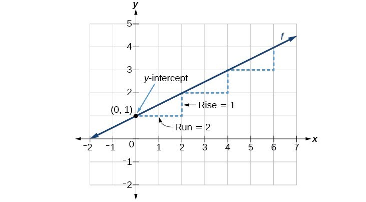
Figure 13

A General Note: Graphical Interpretation of a Linear Function

In the equation [latex]f\left(x\right)=mx+b[/latex]

• b is the y-intercept of the graph and indicates the point (0, b) at which the graph crosses the y-axis.
• m is the slope of the line and indicates the vertical displacement (rise) and horizontal displacement (run) between each successive pair of points. Recall the formula for the slope:

[latex]m=\frac{\text{change in output (rise)}}{\text{change in input (run)}}=\frac{\Delta y}{\Delta x}=\frac{{y}_{2}-{y}_{1}}{{x}_{2}-{x}_{1}}[/latex]

Q & A

Do all linear functions have y-intercepts?

Yes. All linear functions cross the y-axis and therefore have y-intercepts. (Note: A vertical line parallel to the y-axis does not have a y-intercept, but it is not a function.)

How To: Given the equation for a linear function, graph the function using the y-intercept and slope.

1. Evaluate the function at an input value of zero to find the y-intercept.
2. Identify the slope as the rate of change of the input value.
3. Plot the point represented by the y-intercept.
4. Use [latex]\frac{\text{rise}}{\text{run}}[/latex] to determine at least two more points on the line.
5. Sketch the line that passes through the points.

Example 10: Graphing by Using the y-intercept and Slope

Graph [latex]f\left(x\right)=-\frac{2}{3}x+5[/latex] using the y-intercept and slope.

Show Solution

Evaluate the function at x = 0 to find the y-intercept. The output value when x = 0 is 5, so the graph will cross the y-axis at (0,5).

According to the equation for the function, the slope of the line is [latex]-\frac{2}{3}[/latex]. This tells us that for each vertical decrease in the “rise” of –2 units, the “run” increases by 3 units in the horizontal direction. We can now graph the function by first plotting the y-intercept in Figure 3. From the initial value (0, 5) we move down 2 units and to the right 3 units. We can extend the line to the left and right by repeating, and then draw a line through the points.

Figure 14

Analysis of the Solution

The graph slants downward from left to right, which means it has a negative slope as expected.

Try It

Find a point on the graph we drew in Example 10 that has a negative x-value.

Show Solution

Possible answers include [latex]\left(-3,7\right)[/latex], [latex]\left(-6,9\right)[/latex], or [latex]\left(-9,11\right)[/latex].

Try It

Graphing a Linear Function Using Transformations

Another option for graphing is to use transformations of the identity function [latex]f(x)=x[/latex] . A function may be transformed by a shift up, down, left, or right. A function may also be transformed using a reflection, stretch, or compression.

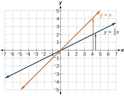
Vertical Stretch or Compression

In the equation [latex]f(x)=mx[/latex], the m is acting as the vertical stretch or compression of the identity function. When m is negative, there is also a vertical reflection of the graph. Notice in Figure 16 that multiplying the equation of [latex]f(x)=x[/latex] by m stretches the graph of f by a factor of m units if m > 1 and compresses the graph of f by a factor of m units if 0 < m < 1. This means the larger the absolute value of m, the steeper the slope.

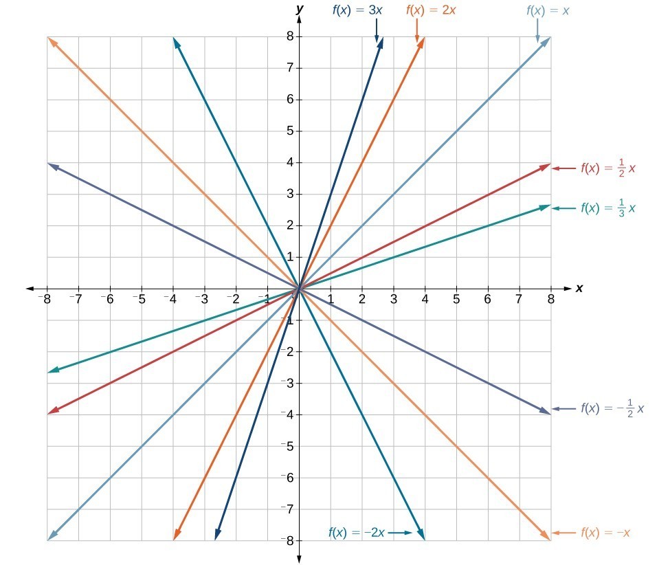
Figure 15. Vertical stretches and compressions and reflections on the function [latex]f\left(x\right)=x[/latex].

Vertical Shift

In [latex]f\left(x\right)=mx+b[/latex], the b acts as the vertical shift, moving the graph up and down without affecting the slope of the line. Notice in Figure 16 that adding a value of b to the equation of [latex]f\left(x\right)=x[/latex] shifts the graph of f a total of b units up if b is positive and |b| units down if b is negative.

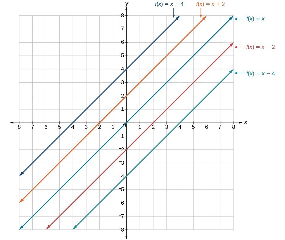
Figure 16. This graph illustrates vertical shifts of the function [latex]f(x)=x[/latex].

Using vertical stretches or compressions along with vertical shifts is another way to look at identifying different types of linear functions. Although this may not be the easiest way to graph this type of function, it is still important to practice each method.

How To: Given the equation of a linear function, use transformations to graph the linear function in the form [latex]f\left(x\right)=mx+b[/latex].

1. Graph [latex]f\left(x\right)=x[/latex].
2. Vertically stretch or compress the graph by a factor m.
3. Shift the graph up or down b units.

Example 11: Graphing by Using Transformations

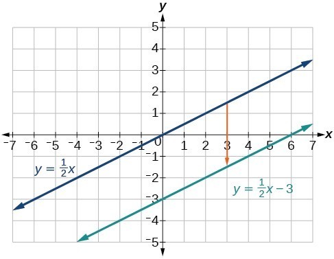
Graph [latex]f\left(x\right)=\frac{1}{2}x - 3[/latex] using transformations.

Show Solution

The equation for the function shows that [latex]m=\frac{1}{2}[/latex] so the identity function is vertically compressed by [latex]\frac{1}{2}[/latex]. The equation for the function also shows that b = –3 so the identity function is vertically shifted down 3 units. First, graph the identity function, and show the vertical compression.

Figure 17. The function, y = x, compressed by a factor of [latex]\frac{1}{2}[/latex].

Then show the vertical shift.

Figure 18. The function [latex]y=\frac{1}{2}x[/latex], shifted down 3 units.

Try It

Graph [latex]f\left(x\right)=4+2x[/latex], using transformations.

Show Solution

Q & A

In Example 3, could we have sketched the graph by reversing the order of the transformations?

No. The order of the transformations follows the order of operations. When the function is evaluated at a given input, the corresponding output is calculated by following the order of operations. This is why we performed the compression first. For example, following the order: Let the input be 2.

[latex]\begin{align}f(2)&=\frac{1}{2}(2)-3 \\ &=1-3 \\ &=-2 \end{align}[/latex]

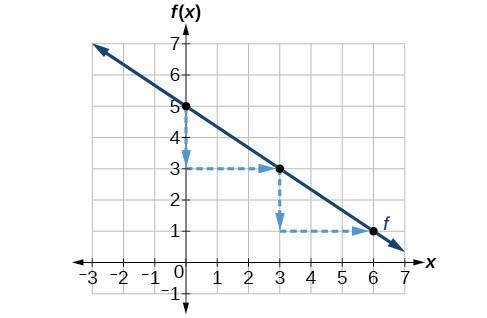
Writing the Equation for a Function from the Graph of a Line

Earlier, we wrote the equation for a linear function from a graph. Now we can extend what we know about graphing linear functions to analyze graphs a little more closely. Begin by taking a look at Figure 21. We can see right away that the graph crosses the y-axis at the point (0, 4) so this is the y-intercept.

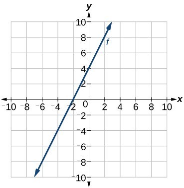
Figure 19

Then we can calculate the slope by finding the rise and run. We can choose any two points, but let’s look at the point (–2, 0). To get from this point to the y-intercept, we must move up 4 units (rise) and to the right 2 units (run). So the slope must be

[latex]m=\frac{\text{rise}}{\text{run}}=\frac{4}{2}=2[/latex]

Substituting the slope and y-intercept into the slope-intercept form of a line gives

[latex]y=2x+4[/latex]

How To: Given a graph of linear function, find the equation to describe the function.

1. Identify the y-intercept of an equation.
2. Choose two points to determine the slope.
3. Substitute the y-intercept and slope into the slope-intercept form of a line.

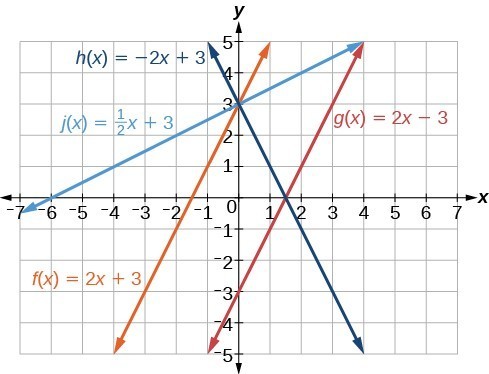
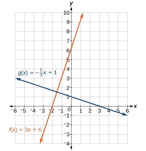
Example 12: Matching Linear Functions to Their Graphs

Match each equation of the linear functions with one of the lines in Figure 20.

1. [latex]f\left(x\right)=2x+3[/latex]
2. [latex]g\left(x\right)=2x - 3[/latex]
3. [latex]h\left(x\right)=-2x+3[/latex]
4. [latex]j\left(x\right)=\frac{1}{2}x+3[/latex]

 

Figure 20

Show Solution

Analyze the information for each function.

1. This function has a slope of 2 and a y-intercept of 3. It must pass through the point (0, 3) and slant upward from left to right. We can use two points to find the slope, or we can compare it with the other functions listed. Function g has the same slope, but a different y-intercept. Lines I and III have the same slant because they have the same slope. Line III does not pass through (0, 3) so f must be represented by line I.
2. This function also has a slope of 2, but a y-intercept of –3. It must pass through the point (0, –3) and slant upward from left to right. It must be represented by line III.
3. This function has a slope of –2 and a y-intercept of 3. This is the only function listed with a negative slope, so it must be represented by line IV because it slants downward from left to right.
4. This function has a slope of [latex]\frac{1}{2}[/latex] and a y-intercept of 3. It must pass through the point (0, 3) and slant upward from left to right. Lines I and II pass through (0, 3), but the slope of j is less than the slope of f so the line for j must be flatter. This function is represented by Line II.

Now we can re-label the lines as in Figure 21.

Figure 21

Finding the x-intercept of a Line

So far, we have been finding the y-intercepts of a function: the point at which the graph of the function crosses the y-axis. A function may also have an x-intercept, which is the x-coordinate of the point where the graph of the function crosses the x-axis. In other words, it is the input value when the output value is zero.

To find the x-intercept, set a function f(x) equal to zero and solve for the value of x. For example, consider the function shown.

[latex]f\left(x\right)=3x - 6[/latex]

Set the function equal to 0 and solve for x.

[latex]\begin{align}&0=3x - 6 \\ &6=3x \\ &2=x \\ &x=2 \end{align}[/latex]

The graph of the function crosses the x-axis at the point (2, 0).

Q & A

Do all linear functions have x-intercepts?

No. However, linear functions of the form y = c, where c is a nonzero real number are the only examples of linear functions with no x-intercept. For example, y = 5 is a horizontal line 5 units above the x-axis. This function has no x-intercepts.

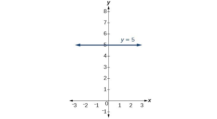
Figure 22

A General Note: x-intercept

The x-intercept of the function is the point where the graph crosses the x-axis. Points on the x-axis have the form (x,0) so we can find x-intercepts by setting f(x) = 0. For a linear function, we solve the equation mx + b = 0

Example 13: Finding an x-intercept

Find the x-intercept of [latex]f\left(x\right)=\frac{1}{2}x - 3[/latex].

Show Solution

Set the function equal to zero to solve for x.

[latex]\begin{align}0&=\frac{1}{2}x - 3\\[1mm] 3&=\frac{1}{2}x\\[1mm] 6&=x\\[1mm] x&=6\end{align}[/latex]

The graph crosses the x-axis at the point (6,0).

Analysis of the Solution

A graph of the function is shown in Figure 23. We can see that the x-intercept is (6, 0) as we expected.

Figure 23. The graph of the linear function [latex]f\left(x\right)=\frac{1}{2}x - 3[/latex].

Try It

Find the x-intercept of [latex]f\left(x\right)=\frac{1}{4}x - 4[/latex].

Show Solution

[latex]\left(16,\text{ 0}\right)[/latex]

Describing Horizontal and Vertical Lines

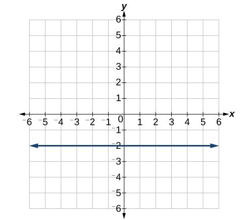
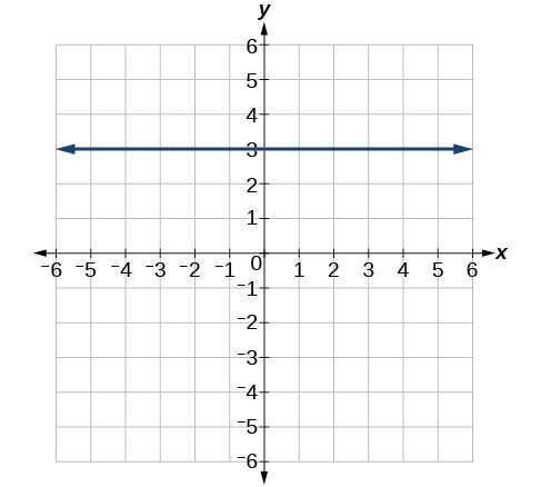
There are two special cases of lines on a graph—horizontal and vertical lines. A horizontal line indicates a constant output, or y-value. In Figure 24, we see that the output has a value of 2 for every input value. The change in outputs between any two points, therefore, is 0. In the slope formula, the numerator is 0, so the slope is 0. If we use m = 0 in the equation [latex]f(x)=mx+b[/latex], the equation simplifies to [latex]f(x)=b[/latex]. In other words, the value of the function is a constant. This graph represents the function [latex]f(x)=2[/latex].

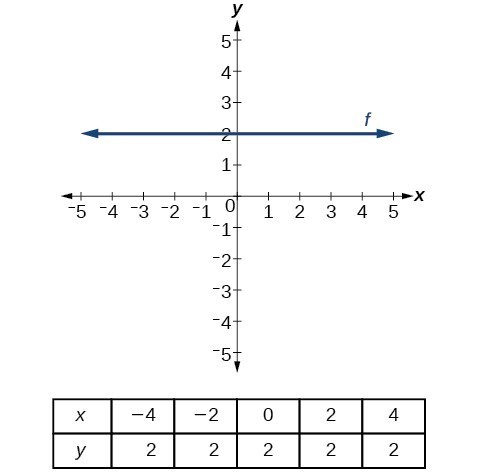
Figure 24. A horizontal line representing the function [latex]f(x)=2[/latex].

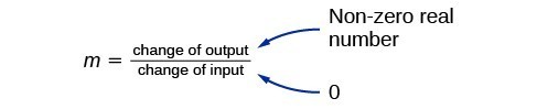
Figure 25

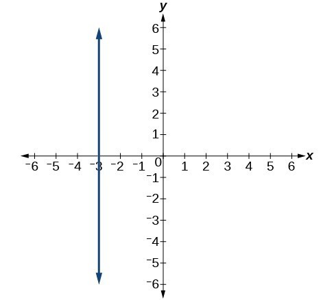
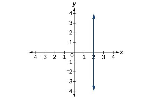
A vertical line indicates a constant input, or x-value. We can see that the input value for every point on the line is 2, but the output value varies. Because this input value is mapped to more than one output value, a vertical line does not represent a function. Notice that between any two points, the change in the input values is zero. In the slope formula, the denominator will be zero, so the slope of a vertical line is undefined.

Notice that a vertical line, such as the one in Figure 26, has an x-intercept, but no y-intercept unless it’s the line x = 0. This graph represents the line x = 2.

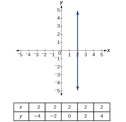
Figure 26. The vertical line, x = 2, which does not represent a function.

A General Note: Horizontal and Vertical Lines

Lines can be horizontal or vertical.

A horizontal line is a line defined by an equation in the form [latex]f(x)=b[/latex].

A vertical line is a line defined by an equation in the form [latex]x=a[/latex].

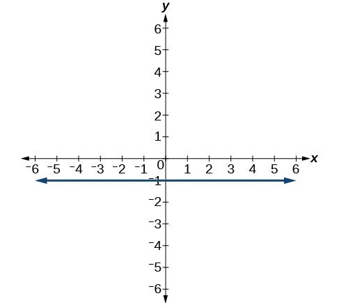
Example 14: Writing the Equation of a Horizontal Line

Write the equation of the line graphed in Figure 27.

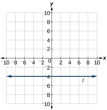
Figure 27

Show Solution

For any x-value, the y-value is –4, so the equation is y = –4.

Example 15: Writing the Equation of a Vertical Line

Write the equation of the line graphed in Figure 28.

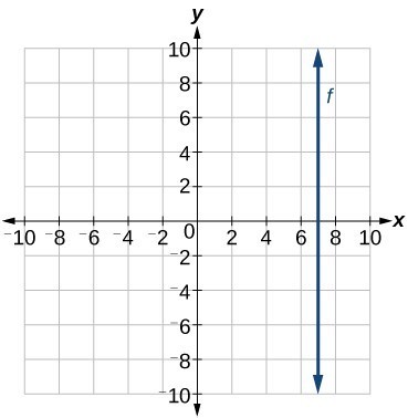
Figure 28

Show Solution

The constant x-value is 7, so the equation is x = 7.

Determining Whether Lines are Parallel or Perpendicular

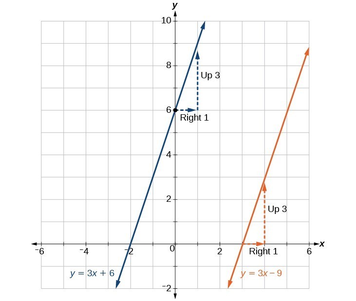
The two lines in Figure 29 are parallel lines: they will never intersect. Notice that they have exactly the same steepness, which means their slopes are identical. The only difference between the two lines is the y-intercept. If we shifted one line vertically toward the y-intercept of the other, they would become the same line.

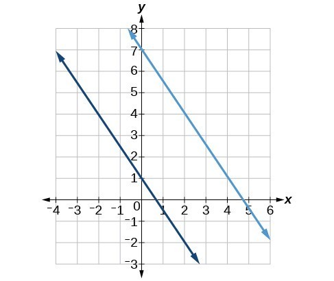
Figure 29 Parallel lines.

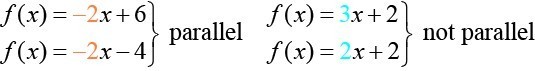
Figure 29

We can determine from their equations whether two lines are parallel by comparing their slopes. If the slopes are the same and the y-intercepts are different, the lines are parallel. If the slopes are different, the lines are not parallel.

Unlike parallel lines, perpendicular lines do intersect. Their intersection forms a right, or 90-degree, angle. The two lines in Figure 30 are perpendicular.

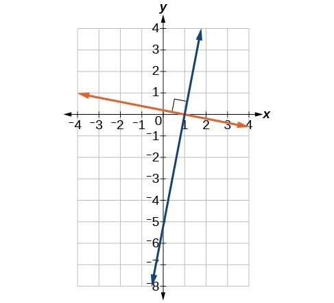
Figure 30. Perpendicular lines.

Perpendicular lines do not have the same slope. The slopes of perpendicular lines are different from one another in a specific way. The slope of one line is the negative reciprocal of the slope of the other line. The product of a number and its reciprocal is 1. So, if [latex]{m}_{1}\text{ and }{m}_{2}[/latex] are negative reciprocals of one another, they can be multiplied together to yield [latex]-1[/latex].

[latex]{m}_{1}{m}_{2}=-1[/latex]

To find the reciprocal of a number, divide 1 by the number. So the reciprocal of 8 is [latex]\frac{1}{8}[/latex], and the reciprocal of [latex]\frac{1}{8}[/latex] is 8. To find the negative reciprocal, first find the reciprocal and then change the sign.

As with parallel lines, we can determine whether two lines are perpendicular by comparing their slopes, assuming that the lines are neither horizontal nor perpendicular. The slope of each line below is the negative reciprocal of the other so the lines are perpendicular.

[latex]\begin{align}&f\left(x\right)=\frac{1}{4}x+2 && \text{negative reciprocal of}\frac{1}{4}\text{ is }-4 \\ &f\left(x\right)=-4x+3 && \text{negative reciprocal of}-4\text{ is }\frac{1}{4} \end{align}[/latex]

The product of the slopes is –1.

[latex]-4\left(\frac{1}{4}\right)=-1[/latex]

A General Note: Parallel and Perpendicular Lines

Two lines are parallel lines if they do not intersect. The slopes of the lines are the same.

[latex]f\left(x\right)={m}_{1}x+{b}_{1}\text{ and }g\left(x\right)={m}_{2}x+{b}_{2}\text{ are parallel if }{m}_{1}={m}_{2}[/latex].

If and only if [latex]{b}_{1}={b}_{2}[/latex] and [latex]{m}_{1}={m}_{2}[/latex], we say the lines coincide. Coincident lines are the same line.

Two lines are perpendicular lines if they intersect at right angles.

[latex]f\left(x\right)={m}_{1}x+{b}_{1}\text{ and }g\left(x\right)={m}_{2}x+{b}_{2}\text{ are perpendicular if }{m}_{1}{m}_{2}=-1,\text{ and so }{m}_{2}=-\frac{1}{{m}_{1}}[/latex].

Example 16: Identifying Parallel and Perpendicular Lines

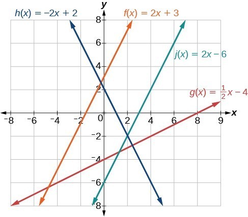
Given the functions below, identify the functions whose graphs are a pair of parallel lines and a pair of perpendicular lines.

[latex]\begin{align}&f\left(x\right)=2x+3 &&h\left(x\right)=-2x+2 \\ &g\left(x\right)=\frac{1}{2}x - 4 && j\left(x\right)=2x - 6 \end{align}[/latex]

Show Solution

Parallel lines have the same slope. Because the functions [latex]f\left(x\right)=2x+3[/latex] and [latex]j\left(x\right)=2x - 6[/latex] each have a slope of 2, they represent parallel lines. Perpendicular lines have negative reciprocal slopes. Because −2 and [latex]\frac{1}{2}[/latex] are negative reciprocals, the equations, [latex]g\left(x\right)=\frac{1}{2}x - 4[/latex] and [latex]h\left(x\right)=-2x+2[/latex] represent perpendicular lines.

Analysis of the Solution

A graph of the lines is shown in Figure 31.

Figure 31. The graph shows that the lines [latex]f\left(x\right)=2x+3[/latex] and [latex]j\left(x\right)=2x - 6[/latex] are parallel, and the lines [latex]g\left(x\right)=\frac{1}{2}x - 4[/latex] and [latex]h\left(x\right)=-2x+2[/latex] are perpendicular.

Writing the Equation of a Line Parallel or Perpendicular to a Given Line

If we know the equation of a line, we can use what we know about slope to write the equation of a line that is either parallel or perpendicular to the given line.

Writing Equations of Parallel Lines

Suppose for example, we are given the following equation.

[latex]f\left(x\right)=3x+1[/latex]

We know that the slope of the line formed by the function is 3. We also know that the y-intercept is (0, 1). Any other line with a slope of 3 will be parallel to f(x). So the lines formed by all of the following functions will be parallel to f(x).

[latex]\begin{align}&g\left(x\right)=3x+6 \\ &h\left(x\right)=3x+1 \\ &p\left(x\right)=3x+\frac{2}{3} \end{align}[/latex]

Suppose then we want to write the equation of a line that is parallel to f and passes through the point (1, 7). We already know that the slope is 3. We just need to determine which value for b will give the correct line. We can begin with the point-slope form of an equation for a line, and then rewrite it in the slope-intercept form.

[latex]\begin{gathered}y-{y}_{1}=m\left(x-{x}_{1}\right) \\ y - 7=3\left(x - 1\right) \\ y - 7=3x - 3 \\ y=3x+4 \end{gathered}[/latex]

So [latex]g(x)=3x+4[/latex] is parallel to [latex]f(x)=3x+1[/latex] and passes through the point (1,7).

How To: Given the equation of a function and a point through which its graph passes, write the equation of a line parallel to the given line that passes through the given point.

1. Find the slope of the function.
2. Substitute the given values into either the general point-slope equation or the slope-intercept equation for a line.
3. Simplify.

Example 17: Finding a Line Parallel to a Given Line

Find a line parallel to the graph of [latex]f\left(x\right)=3x+6[/latex] that passes through the point (3,0).

Show Solution

The slope of the given line is 3. If we choose the slope-intercept form, we can substitute m = 3, x = 3, and f(x) = 0 into the slope-intercept form to find the y-intercept.

[latex]\begin{gathered}g\left(x\right)=3x+b \\ 0=3\left(3\right)+b \\ b=-9 \end{gathered}[/latex]

The line parallel to f(x) that passes through (3, 0) is [latex]g\left(x\right)=3x - 9[/latex].

Analysis of the Solution

We can confirm that the two lines are parallel by graphing them. Figure 32 shows that the two lines will never intersect.

Figure 32

Writing Equations of Perpendicular Lines

We can use a very similar process to write the equation for a line perpendicular to a given line. Instead of using the same slope, however, we use the negative reciprocal of the given slope. Suppose we are given the following function:

[latex]f\left(x\right)=2x+4[/latex]

The slope of the line is 2, and its negative reciprocal is [latex]-\frac{1}{2}[/latex]. Any function with a slope of [latex]-\frac{1}{2}[/latex] will be perpendicular to f(x). So the lines formed by all of the following functions will be perpendicular to f(x).

[latex]\begin{align}&g\left(x\right)=-\frac{1}{2}x+4 \\ &h\left(x\right)=-\frac{1}{2}x+2 \\ &p\left(x\right)=-\frac{1}{2}x-\frac{1}{2} \end{align}[/latex]

As before, we can narrow down our choices for a particular perpendicular line if we know that it passes through a given point. Suppose then we want to write the equation of a line that is perpendicular to f(x) and passes through the point (4, 0). We already know that the slope is [latex]-\frac{1}{2}[/latex]. Now we can use the point to find the y-intercept by substituting the given values into the slope-intercept form of a line and solving for b.

[latex]\begin{gathered}g\left(x\right)=mx+b \\ 0=-\frac{1}{2}\left(4\right)+b \\ 0=-2+b \\ 2=b \\ b=2 \end{gathered}[/latex]

The equation for the function with a slope of [latex]-\frac{1}{2}[/latex] and a y-intercept of 2 is

[latex]g\left(x\right)=-\frac{1}{2}x+2[/latex].

So [latex]g\left(x\right)=-\frac{1}{2}x+2[/latex] is perpendicular to [latex]f\left(x\right)=2x+4[/latex] and passes through the point (4,0). Be aware that perpendicular lines may not look obviously perpendicular on a graphing calculator unless we use the square zoom feature.

Q & A

A horizontal line has a slope of zero and a vertical line has an undefined slope. These two lines are perpendicular, but the product of their slopes is not –1. Doesn’t this fact contradict the definition of perpendicular lines?

No. For two perpendicular linear functions, the product of their slopes is –1. However, a vertical line is not a function so the definition is not contradicted.

How To: Given the equation of a function and a point through which its graph passes, write the equation of a line perpendicular to the given line.

1. Find the slope of the function.
2. Determine the negative reciprocal of the slope.
3. Substitute the new slope and the values for x and y from the coordinate pair provided into [latex]g\left(x\right)=mx+b[/latex].
4. Solve for b.
5. Write the equation for the line.

Example 18: Finding the Equation of a Perpendicular Line

Find the equation of a line perpendicular to [latex]f\left(x\right)=3x+3[/latex] that passes through the point (3,0).

Show Solution

The original line has slope m = 3, so the slope of the perpendicular line will be its negative reciprocal, or [latex]-\frac{1}{3}[/latex]. Using this slope and the given point, we can find the equation for the line.

[latex]\begin{gathered}g\left(x\right)=-\frac{1}{3}x+b \\ 0=-\frac{1}{3}\left(3\right)+b \\ 1=b \\ b=1 \end{gathered}[/latex]

The line perpendicular to f(x) that passes through (3, 0) is [latex]g\left(x\right)=-\frac{1}{3}x+1[/latex].

Analysis of the Solution

A graph of the two lines is shown in Figure 33.

Figure 33

Try It

Given the function [latex]h\left(x\right)=2x - 4[/latex], write an equation for the line passing through (0, 0) that is

a. parallel to h(x)
b. perpendicular to h(x)

Show Solution

a. [latex]f\left(x\right)=2x[/latex]
b. [latex]g\left(x\right)=-\frac{1}{2}x[/latex]

Try It

How To: Given two points on a line and a third point, write the equation of the perpendicular line that passes through the point.

1. Determine the slope of the line passing through the points.
2. Find the negative reciprocal of the slope.
3. Use the slope-intercept form or point-slope form to write the equation by substituting the known values.
4. Simplify.

Example 19: Finding the Equation of a Line Perpendicular to a Given Line Passing through a Point

A line passes through the points (–2, 6) and (4, 5). Find the equation of a perpendicular line that passes through the point (4, 5).

Show Solution

From the two points of the given line, we can calculate the slope of that line.

[latex]\begin{align}{m}_{1}&=\frac{5 - 6}{4-\left(-2\right)} \\ &=\frac{-1}{6} \\ &=-\frac{1}{6} \end{align}[/latex]

Find the negative reciprocal of the slope.

[latex]\begin{align}{m}_{2}&=\frac{-1}{-\frac{1}{6}} \\ &=-1\left(-\frac{6}{1}\right) \\ &=6 \end{align}[/latex]

We can then solve for the y-intercept of the line passing through the point (4, 5).

[latex]\begin{gathered}g\left(x\right)=6x+b \\ 5=6\left(4\right)+b \\ 5=24+b \\ -19=b \\ b=-19 \end{gathered}[/latex]

The equation for the line that is perpendicular to the line passing through the two given points and also passes through point (4, 5) is

[latex]y=6x - 19[/latex]

Try It

A line passes through the points, (–2, –15) and (2, –3). Find the equation of a perpendicular line that passes through the point, (6, 4).

Show Solution

[latex]y=-\frac{1}{3}x+6[/latex]

Key Equations

slope-intercept form of a line	[latex]f\left(x\right)=mx+b[/latex]
slope	[latex]m=\frac{\text{change in output (rise)}}{\text{change in input (run)}}=\frac{\Delta y}{\Delta x}=\frac{{y}_{2}-{y}_{1}}{{x}_{2}-{x}_{1}}[/latex]
point-slope form of a line	[latex]y-{y}_{1}=m\left(x-{x}_{1}\right)[/latex]

Key Concepts

• • The ordered pairs given by a linear function represent points on a line.
  • Linear functions can be represented in words, function notation, tabular form, and graphical form.
  • The rate of change of a linear function is also known as the slope.
  • An equation in the slope-intercept form of a line includes the slope and the initial value of the function.
  • The initial value, or y-intercept, is the output value when the input of a linear function is zero. It is the y-value of the point at which the line crosses the y-axis.
  • An increasing linear function results in a graph that slants upward from left to right and has a positive slope.
  • A decreasing linear function results in a graph that slants downward from left to right and has a negative slope.
  • A constant linear function results in a graph that is a horizontal line.
  • Analyzing the slope within the context of a problem indicates whether a linear function is increasing, decreasing, or constant.
  • The slope of a linear function can be calculated by dividing the difference between y-values by the difference in corresponding x-values of any two points on the line.
  • The slope and initial value can be determined given a graph or any two points on the line.
  • One type of function notation is the slope-intercept form of an equation.
  • The point-slope form is useful for finding a linear equation when given the slope of a line and one point.
  • The point-slope form is also convenient for finding a linear equation when given two points through which a line passes.
  • The equation for a linear function can be written if the slope m and initial value b are known.
  • A linear function can be used to solve real-world problems.
  • A linear function can be written from tabular form.
  • Linear functions may be graphed by plotting points or by using the y-intercept and slope.
  • Graphs of linear functions may be transformed by using shifts up, down, left, or right, as well as through stretches, compressions, and reflections.
  • The y-intercept and slope of a line may be used to write the equation of a line.
  • The x-intercept is the point at which the graph of a linear function crosses the x-axis.
  • Horizontal lines are written in the form, f(x) = b.
  • Vertical lines are written in the form, x = b.
  • Parallel lines have the same slope.
  • Perpendicular lines have negative reciprocal slopes, assuming neither is vertical.
  • A line parallel to another line, passing through a given point, may be found by substituting the slope value of the line and the x– and y-values of the given point into the equation, [latex]f(x)=mx+b[/latex], and using the b that results. Similarly, the point-slope form of an equation can also be used.
  • A line perpendicular to another line, passing through a given point, may be found in the same manner, with the exception of using the negative reciprocal slope.

Glossary

decreasing linear function

a function with a negative slope: If [latex]f\left(x\right)=mx+b, \text{then } m<0[/latex].

horizontal line

a line defined by [latex]f(x)=b[/latex], where b is a real number. The slope of a horizontal line is 0.

increasing linear function

a function with a positive slope: If [latex]f\left(x\right)=mx+b, \text{then } m>0[/latex].

linear function

a function with a constant rate of change that is a polynomial of degree 1, and whose graph is a straight line

point-slope form

the equation for a line that represents a linear function of the form [latex]y-{y}_{1}=m\left(x-{x}_{1}\right)[/latex]

slope

the ratio of the change in output values to the change in input values; a measure of the steepness of a line

slope-intercept form

the equation for a line that represents a linear function in the form [latex]f\left(x\right)=mx+b[/latex]

vertical line

a line defined by x = a, where a is a real number. The slope of a vertical line is undefined.

x-intercept

the point on the graph of a linear function when the output value is 0; the point at which the graph crosses the horizontal axis

y-intercept

the value of a function when the input value is zero; also known as initial value

Parallel Lines

two or more lines with the same slope

Perpendicular Lines

two lines that intersect at right angles and have slopes that are negative reciprocals of each other

 

Section 1.3 Homework Exercises

1. If the graphs of two linear functions are parallel, describe the relationship between the slopes and the y-intercepts.

2. If the graphs of two linear functions are perpendicular, describe the relationship between the slopes and the y-intercepts.

3. Terry is skiing down a steep hill. Terry’s elevation, E(t), in feet after t seconds is given by [latex]E\left(t\right)=3000-70t[/latex]. Write a complete sentence describing Terry’s starting elevation and how it is changing over time.

4. Maria is climbing a mountain. Maria’s elevation, E(t), in feet after t minutes is given by [latex]E\left(t\right)=1200+40t[/latex]. Write a complete sentence describing Maria’s starting elevation and how it is changing over time.

5. Jessica is walking home from a friend’s house. After 2 minutes she is 1.4 miles from home. Twelve minutes after leaving, she is 0.9 miles from home. What is her rate in miles per hour?

6. Sonya is currently 10 miles from home and is walking farther away at 2 miles per hour. Write an equation for her distance from home t hours from now.

7. A boat is 100 miles away from the marina, sailing directly toward it at 10 miles per hour. Write an equation for the distance of the boat from the marina after t hours.

8. Timmy goes to the fair with $40. Each ride costs $2. How much money will he have left after riding [latex]n[/latex] rides?

For the following exercises, determine whether the equation of the curve can be written as a linear equation.

9. [latex]y=\frac{1}{4}x+6[/latex]

10. [latex]y=3x - 5[/latex]

11. [latex]y=3{x}^{2}-2[/latex]

12. [latex]3x+5y=15[/latex]

13. [latex]3{x}^{2}+5y=15[/latex]

14. [latex]3x+5{y}^{2}=15[/latex]

15. [latex]-2{x}^{2}+3{y}^{2}=6[/latex]

16. [latex]-\frac{x - 3}{5}=2y[/latex]

For the following exercises, determine whether each function is increasing or decreasing.

17. [latex]f\left(x\right)=4x+3[/latex]

18. [latex]g\left(x\right)=5x+6[/latex]

19. [latex]a\left(x\right)=5 - 2x[/latex]

20. [latex]b\left(x\right)=8 - 3x[/latex]

21. [latex]h\left(x\right)=-2x+4[/latex]

22. [latex]k\left(x\right)=-4x+1[/latex]

23. [latex]j\left(x\right)=\frac{1}{2}x - 3[/latex]

24. [latex]p\left(x\right)=\frac{1}{4}x - 5[/latex]

25. [latex]n\left(x\right)=-\frac{1}{3}x - 2[/latex]

26. [latex]m\left(x\right)=-\frac{3}{8}x+3[/latex]

For the following exercises, find the slope of the line that passes through the two given points.

27. [latex]\left(2,\text{ }4\right)[/latex] and [latex]\left(4,\text{ 10}\right)[/latex]

28. [latex]\left(1,\text{ 5}\right)[/latex] and [latex]\left(4,\text{ 11}\right)[/latex]

29. [latex]\left(-1,\text{4}\right)[/latex] and [latex]\left(5,\text{2}\right)[/latex]

30. [latex]\left(8,-2\right)[/latex] and [latex]\left(4,6\right)[/latex]

31. [latex]\left(6,\text{ }11\right)[/latex] and [latex]\left(-4, 3\right)[/latex]

For the following exercises, given each set of information, find a linear equation satisfying the conditions, if possible.

32. [latex]f\left(-5\right)=-4[/latex], and [latex]f\left(5\right)=2[/latex]

33. [latex]f\left(-1\right)=4[/latex] and [latex]f\left(5\right)=1[/latex]

34. [latex]\left(2,4\right)[/latex] and [latex]\left(4,10\right)[/latex]

35. Passes through [latex]\left(1,5\right)[/latex] and [latex]\left(4,11\right)[/latex]

36. Passes through [latex]\left(-1,\text{ 4}\right)[/latex] and [latex]\left(5,\text{ 2}\right)[/latex]

37. Passes through [latex]\left(-2,\text{ 8}\right)[/latex] and [latex]\left(4,\text{ 6}\right)[/latex]

38. x intercept at [latex]\left(-2,\text{ 0}\right)[/latex] and y intercept at [latex]\left(0,-3\right)[/latex]

39. x intercept at [latex]\left(-5,\text{ 0}\right)[/latex] and y intercept at [latex]\left(0,\text{ 4}\right)[/latex]

For the following exercises, find the slope of the lines graphed.

40.

41.

42.

For the following exercises, write an equation for the lines graphed.

43.

44.

45.

46.

47.

48.

For the following exercises, which of the tables could represent a linear function? For each that could be linear, find a linear equation that models the data.

49.

x	0	5	10	15
g(x)	5	–10	–25	–40

50.

x	0	5	10	15
h(x)	5	30	105	230

51.

x	0	5	10	15
f(x)	–5	20	45	70

52.

x	5	10	20	25
k(x)	28	13	58	73

53.

x	0	2	4	6
g(x)	6	–19	–44	–69

54.

x	2	4	6	8
f(x)	–4	16	36	56

55.

x	2	4	6	8
f(x)	–4	16	36	56

56.

x	0	2	6	8
k(x)	6	31	106	231

57. Find the value of x if a linear function goes through the following points and has the following slope: [latex]\left(x,2\right),\left(-4,6\right),m=3[/latex]

58. Find the value of y if a linear function goes through the following points and has the following slope: [latex]\left(10,y\right),\left(25,100\right),m=-5[/latex]

59. Find the equation of the line that passes through the following points: [latex]\left(a,\text{ }b\right)[/latex] and [latex]\left(a,\text{ }b+1\right)[/latex]

60. Find the equation of the line that passes through the following points: [latex]\left(2a,\text{ }b\right)[/latex] and [latex]\left(a,\text{ }b+1\right)[/latex]

61. Find the equation of the line that passes through the following points: [latex]\left(a,\text{ }0\right)[/latex] and [latex]\left(c,\text{ }d\right)[/latex]

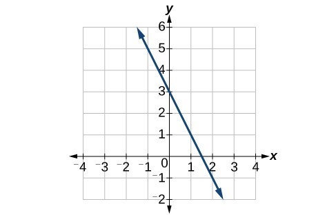
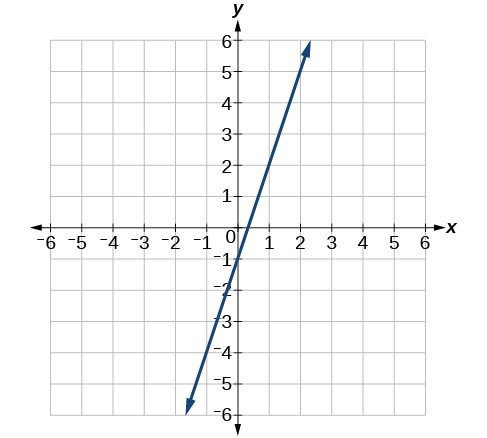
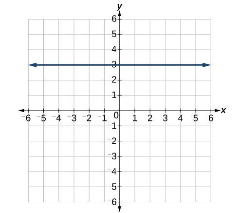
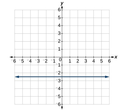
For the following exercises, match the given linear equation with its graph.

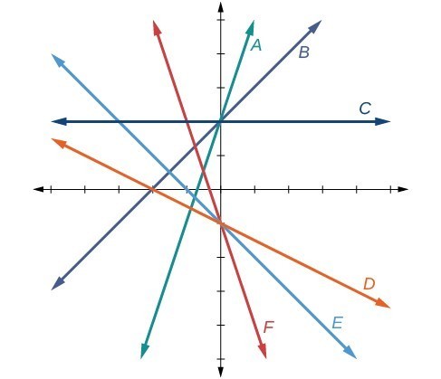
62. [latex]f\left(x\right)=-x - 1[/latex]

63. [latex]f\left(x\right)=-2x - 1[/latex]

64. [latex]f\left(x\right)=-\frac{1}{2}x - 1[/latex]

65. [latex]f\left(x\right)=2[/latex]

66. [latex]f\left(x\right)=2+x[/latex]

67. [latex]f\left(x\right)=3x+2[/latex]

For the following exercises, sketch a line with the given features.

68. An x-intercept of [latex]\left(-\text{4},\text{ 0}\right)[/latex] and y-intercept of [latex]\left(0,\text{ -2}\right)[/latex]

69. An x-intercept of [latex]\left(-\text{2},\text{ 0}\right)[/latex] and y-intercept of [latex]\left(0,\text{ 4}\right)[/latex]

70. A y-intercept of [latex]\left(0,\text{ 7}\right)[/latex] and slope [latex]-\frac{3}{2}[/latex]

71. A y-intercept of [latex]\left(0,\text{ 3}\right)[/latex] and slope [latex]\frac{2}{5}[/latex]

72. Passing through the points [latex]\left(-\text{6},\text{ -2}\right)[/latex] and [latex]\left(\text{6},\text{ -6}\right)[/latex]

73. Passing through the points [latex]\left(-\text{3},\text{ -4}\right)[/latex] and [latex]\left(\text{3},\text{ 0}\right)[/latex]

For the following exercises, sketch the graph of each equation.

74. [latex]f\left(x\right)=-2x - 1[/latex]

75. [latex]g\left(x\right)=-3x+2[/latex]

76. [latex]h\left(x\right)=\frac{1}{3}x+2[/latex]

77. [latex]k\left(x\right)=\frac{2}{3}x - 3[/latex]

78. [latex]f\left(t\right)=3+2t[/latex]

79. [latex]p\left(t\right)=-2+3t[/latex]

80. [latex]x=3[/latex]

81. [latex]x=-2[/latex]

82. [latex]r\left(x\right)=4[/latex]

83. [latex]q\left(x\right)=3[/latex]

84. [latex]4x=-9y+36[/latex]

85. [latex]\frac{x}{3}-\frac{y}{4}=1[/latex]

86. [latex]3x - 5y=15[/latex]

87. [latex]3x=15[/latex]

88. [latex]3y=12[/latex]

89. If [latex]g\left(x\right)[/latex] is the transformation of [latex]f\left(x\right)=x[/latex] after a vertical compression by [latex]\frac{3}{4}[/latex], a shift right by 2, and a shift down by 4

a. Write an equation for [latex]g\left(x\right)[/latex].

b. What is the slope of this line?

c. Find the y-intercept of this line.

90. If [latex]g\left(x\right)[/latex] is the transformation of [latex]f\left(x\right)=x[/latex] after a vertical compression by [latex]\frac{1}{3}[/latex], a shift left by 1, and a shift up by 3

a. Write an equation for [latex]g\left(x\right)[/latex].

b. What is the slope of this line?

c. Find the y-intercept of this line.

For the following exercises, write the equation of the line shown in the graph.

91.

92.

93.

94.

95. Explain how to find the input variable in a word problem that uses a linear function.

96. Explain how to find the output variable in a word problem that uses a linear function.

97. Explain how to interpret the initial value in a word problem that uses a linear function.

98. Explain how to determine the slope in a word problem that uses a linear function.

99. Explain how to find a line perpendicular to a linear function that passes through a given point.

For the following exercises, determine whether the lines given by the equations below are parallel, perpendicular, or neither parallel nor perpendicular:

100. [latex]\begin{cases}4x - 7y=10\hfill \\ 7x+4y=1\hfill \end{cases}[/latex]

101. [latex]\begin{cases}3y+x=12\\ -y=8x+1\end{cases}[/latex]

102. [latex]\begin{cases}3y+4x=12\\ -6y=8x+1\end{cases}[/latex]

103. [latex]\begin{cases}6x - 9y=10\\ 3x+2y=1\end{cases}[/latex]

104. [latex]\begin{cases}y=\frac{2}{3}x+1\\ 3x+2y=1\end{cases}[/latex]

105. [latex]\begin{cases}y=\frac{3}{4}x+1\\ -3x+4y=1\end{cases}[/latex]

For the following exercises, use the descriptions of each pair of lines given below to find the slopes of Line 1 and Line 2. Is each pair of lines parallel, perpendicular, or neither?

106. Line 1: Passes through [latex]\left(0,6\right)[/latex] and [latex]\left(3,-24\right)[/latex]
Line 2: Passes through [latex]\left(-1,19\right)[/latex] and [latex]\left(8,-71\right)[/latex]

107. Line 1: Passes through [latex]\left(-8,-55\right)[/latex] and [latex]\left(10,89\right)[/latex]
Line 2: Passes through [latex]\left(9,-44\right)[/latex] and [latex]\left(4,-14\right)[/latex]

108. Line 1: Passes through [latex]\left(2,3\right)[/latex] and [latex]\left(4,-1\right)[/latex]
Line 2: Passes through [latex]\left(6,3\right)[/latex] and [latex]\left(8,5\right)[/latex]

109. Line 1: Passes through [latex]\left(1,7\right)[/latex] and [latex]\left(5,5\right)[/latex]
Line 2: Passes through [latex]\left(-1,-3\right)[/latex] and [latex]\left(1,1\right)[/latex]

110. Line 1: Passes through [latex]\left(0,5\right)[/latex] and [latex]\left(3,3\right)[/latex]
Line 2: Passes through [latex]\left(1,-5\right)[/latex] and [latex]\left(3,-2\right)[/latex]

111. Write an equation for a line parallel to [latex]g\left(x\right)=3x - 1[/latex] and passing through the point [latex]\left(4,9\right)[/latex].

112. Write an equation for a line parallel to [latex]f\left(x\right)=-5x - 3[/latex] and passing through the point [latex]\left(2,\text{ -}12\right)[/latex].

113. Write an equation for a line perpendicular to [latex]p\left(t\right)=3t+4[/latex] and passing through the point [latex]\left(3,1\right)[/latex].

114. Write an equation for a line perpendicular to [latex]h\left(t\right)=-2t+4[/latex] and passing through the point [latex]\left(\text{-}4,\text{ -}1\right)[/latex].