Learning Outcomes
- Find a rectangular equation for a curve defined parametrically.
- Find parametric equations for curves defined by rectangular equations.
- Graph plane curves described by parametric equations by plotting points.
- Graph parametric equations.
Consider the path a moon follows as it orbits a planet, which simultaneously rotates around the sun, as seen in Figure 1. At any moment, the moon is located at a particular spot relative to the planet. But how do we write and solve the equation for the position of the moon when the distance from the planet, the speed of the moon’s orbit around the planet, and the speed of rotation around the sun are all unknowns? We can solve only for one variable at a time.
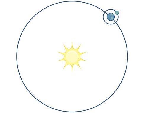
Figure 1
In this section, we will consider sets of equations given by [latex]x\left(t\right)[/latex] and [latex]y\left(t\right)[/latex] where [latex]t[/latex] is the independent variable of time. We can use these parametric equations in a number of applications when we are looking for not only a particular position but also the direction of the movement. As we trace out successive values of [latex]t[/latex], the orientation of the curve becomes clear. This is one of the primary advantages of using parametric equations: we are able to trace the movement of an object along a path according to time. We begin this section with a look at the basic components of parametric equations and what it means to parameterize a curve. Then we will learn how to eliminate the parameter, translate the equations of a curve defined parametrically into rectangular equations, and find the parametric equations for curves defined by rectangular equations.
Parameterizing a Curve
When an object moves along a curve—or curvilinear path—in a given direction and in a given amount of time, the position of the object in the plane is given by the x-coordinate and the y-coordinate. However, both [latex]x[/latex] and [latex]y[/latex]
vary over time and so are functions of time. For this reason, we add another variable, the parameter, upon which both [latex]x[/latex] and [latex]y[/latex] are dependent functions. In the example in the section opener, the parameter is time, [latex]t[/latex]. The [latex]x[/latex] position of the moon at time, [latex]t[/latex], is represented as the function [latex]x\left(t\right)[/latex], and the [latex]y[/latex] position of the moon at time, [latex]t[/latex], is represented as the function [latex]y\left(t\right)[/latex]. Together, [latex]x\left(t\right)[/latex] and [latex]y\left(t\right)[/latex] are called parametric equations, and generate an ordered pair [latex]\left(x\left(t\right),y\left(t\right)\right)[/latex]. Parametric equations primarily describe motion and direction.
When we parameterize a curve, we are translating a single equation in two variables, such as [latex]x[/latex] and [latex]y[/latex], into an equivalent pair of equations in three variables, [latex]x,y[/latex], and [latex]t[/latex]. One of the reasons we parameterize a curve is because the parametric equations yield more information: specifically, the direction of the object’s motion over time.
When we graph parametric equations, we can observe the individual behaviors of [latex]x[/latex] and of [latex]y[/latex]. There are a number of shapes that cannot be represented in the form [latex]y=f\left(x\right)[/latex], meaning that they are not functions. For example, consider the graph of a circle, given as [latex]{r}^{2}={x}^{2}+{y}^{2}[/latex]. Solving for [latex]y[/latex] gives [latex]y=\pm \sqrt{{r}^{2}-{x}^{2}}[/latex], or two equations: [latex]{y}_{1}=\sqrt{{r}^{2}-{x}^{2}}[/latex] and [latex]{y}_{2}=-\sqrt{{r}^{2}-{x}^{2}}[/latex]. If we graph [latex]{y}_{1}[/latex] and [latex]{y}_{2}[/latex] together, the graph will not pass the vertical line test, as shown in Figure 2. Thus, the equation for the graph of a circle is not a function.
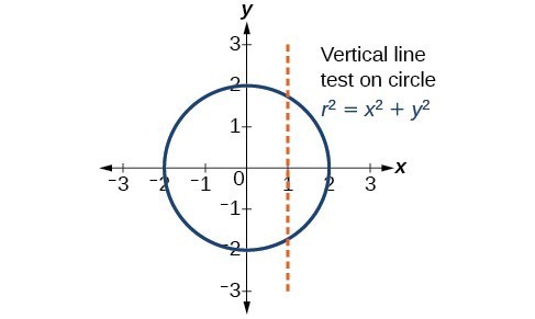
Figure 2
However, if we were to graph each equation on its own, each one would pass the vertical line test and therefore would represent a function. In some instances, the concept of breaking up the equation for a circle into two functions is similar to the concept of creating parametric equations, as we use two functions to produce a non-function. This will become clearer as we move forward.
A General Note: Parametric Equations
Suppose [latex]t[/latex] is a number on an interval, [latex]I[/latex]. The set of ordered pairs, [latex]\left(x\left(t\right),y\left(t\right)\right)[/latex], where [latex]x=f\left(t\right)[/latex] and [latex]y=g\left(t\right)[/latex], forms a plane curve based on the parameter [latex]t[/latex]. The equations [latex]x=f\left(t\right)[/latex] and [latex]y=g\left(t\right)[/latex] are the parametric equations.
Example 1: Parameterizing a Curve
Parameterize the curve [latex]y={x}^{2}-1[/latex] letting [latex]x\left(t\right)=t[/latex]. Graph both equations.

Try It
Construct a table of values and plot the parametric equations: [latex]x\left(t\right)=t - 3,y\left(t\right)=2t+4;-1\le t\le 2[/latex].

Example 2: Finding a Pair of Parametric Equations
Find a pair of parametric equations that models the graph of [latex]y=1-{x}^{2}[/latex], using the parameter [latex]x\left(t\right)=t[/latex]. Plot some points and sketch the graph.

Try It
Parameterize the curve given by [latex]x={y}^{3}-2y[/latex].
Example 3: Finding Parametric Equations That Model Given Criteria
An object travels at a steady rate along a straight path [latex]\left(-5,3\right)[/latex] to [latex]\left(3,-1\right)[/latex] in the same plane in four seconds. The coordinates are measured in meters. Find parametric equations for the position of the object.

Methods for Finding Cartesian and Polar Equations from Curves
In many cases, we may have a pair of parametric equations but find that it is simpler to draw a curve if the equation involves only two variables, such as [latex]x[/latex] and [latex]y[/latex]. Eliminating the parameter is a method that may make graphing some curves easier. However, if we are concerned with the mapping of the equation according to time, then it will be necessary to indicate the orientation of the curve as well. There are various methods for eliminating the parameter [latex]t[/latex] from a set of parametric equations; not every method works for every type of equation. Here we will review the methods for the most common types of equations.
Eliminating the Parameter from Polynomial, Exponential, and Logarithmic Equations
For polynomial, exponential, or logarithmic equations expressed as two parametric equations, we choose the equation that is most easily manipulated and solve for [latex]t[/latex]. We substitute the resulting expression for [latex]t[/latex] into the second equation. This gives one equation in [latex]x[/latex] and [latex]y[/latex].
Example 4: Eliminating the Parameter in Polynomials
Given [latex]x\left(t\right)={t}^{2}+1[/latex] and [latex]y\left(t\right)=2+t[/latex], eliminate the parameter, and write the parametric equations as a Cartesian equation.

Try It
Given the equations below, eliminate the parameter and write as a rectangular equation for [latex]y[/latex] as a function of [latex]x[/latex].
[latex]\begin{align}&x\left(t\right)=2{t}^{2}+6 \\ &y\left(t\right)=5-t\end{align}[/latex]
Try It
Example 5: Eliminating the Parameter in Exponential Equations
Eliminate the parameter and write as a Cartesian equation: [latex]x\left(t\right)={e}^{-t}[/latex] and [latex]y\left(t\right)=3{e}^{t},t>0[/latex].

Example 6: Eliminating the Parameter in Logarithmic Equations
Eliminate the parameter and write as a Cartesian equation: [latex]x\left(t\right)=\sqrt{t}+2[/latex] and [latex]y\left(t\right)=\mathrm{log}\left(t\right)[/latex].
Try It
Eliminate the parameter and write as a rectangular equation.
[latex]\begin{align}&x\left(t\right)={t}^{2} \\ &y\left(t\right)=\mathrm{ln}t,t>0\end{align}[/latex]
Eliminating the Parameter from Trigonometric Equations
Eliminating the parameter from trigonometric equations is a straightforward substitution. We can use a few of the familiar trigonometric identities and the Pythagorean Theorem.
First, we use the identities:
[latex]\begin{gathered}x\left(t\right)=a\cos t\\ y\left(t\right)=b\sin t\end{gathered}[/latex]
Solving for [latex]\cos t[/latex] and [latex]\sin t[/latex], we have
[latex]\begin{gathered}\frac{x}{a}=\cos t\\ \frac{y}{b}=\sin t\end{gathered}[/latex]
Then, use the Pythagorean Theorem:
[latex]{\cos }^{2}t+{\sin }^{2}t=1[/latex]
Substituting gives
Example 7: Eliminating the Parameter from a Pair of Trigonometric Parametric Equations
Eliminate the parameter from the given pair of trigonometric equations where [latex]0\le t\le 2\pi[/latex] and sketch the graph.
[latex]\begin{align}&x\left(t\right)=4\cos t\\ &y\left(t\right)=3\sin t\end{align}[/latex]

Try It
Eliminate the parameter from the given pair of parametric equations and write as a Cartesian equation:
[latex]x\left(t\right)=2\cos t[/latex] and [latex]y\left(t\right)=3\sin t[/latex].
Try It
When we are given a set of parametric equations and need to find an equivalent Cartesian equation, we are essentially “eliminating the parameter.” However, there are various methods we can use to rewrite a set of parametric equations as a Cartesian equation. The simplest method is to set one equation equal to the parameter, such as [latex]x\left(t\right)=t[/latex]. In this case, [latex]y\left(t\right)[/latex] can be any expression. For example, consider the following pair of equations.
Rewriting this set of parametric equations is a matter of substituting [latex]x[/latex] for [latex]t[/latex]. Thus, the Cartesian equation is [latex]y={x}^{2}-3[/latex].
Example 8: Finding a Cartesian Equation Using Alternate Methods
Use two different methods to find the Cartesian equation equivalent to the given set of parametric equations.
[latex]\begin{align}&x\left(t\right)=3t - 2 \\ &y\left(t\right)=t+1 \end{align}[/latex]
Try It
Write the given parametric equations as a Cartesian equation: [latex]x\left(t\right)={t}^{3}[/latex] and [latex]y\left(t\right)={t}^{6}[/latex].
Finding Parametric Equations for Curves Defined by Rectangular Equations
Although we have just shown that there is only one way to interpret a set of parametric equations as a rectangular equation, there are multiple ways to interpret a rectangular equation as a set of parametric equations. Any strategy we may use to find the parametric equations is valid if it produces equivalency. In other words, if we choose an expression to represent [latex]x[/latex], and then substitute it into the [latex]y[/latex] equation, and it produces the same graph over the same domain as the rectangular equation, then the set of parametric equations is valid. If the domain becomes restricted in the set of parametric equations, and the function does not allow the same values for [latex]x[/latex] as the domain of the rectangular equation, then the graphs will be different.
The following video shows examples of how to find Cartesian representations of parametric equations of different kinds.
Example 9: Finding a Set of Parametric Equations for Curves Defined by Rectangular Equations
Find a set of equivalent parametric equations for [latex]y={\left(x+3\right)}^{2}+1[/latex].

Graphing Parametric Equations by Plotting Points
In lieu of a graphing calculator or a computer graphing program, plotting points to represent the graph of an equation is the standard method. As long as we are careful in calculating the values, point-plotting is highly dependable.
How To: Given a pair of parametric equations, sketch a graph by plotting points.
- Construct a table with three columns: [latex]t,x\left(t\right),\text{and}y\left(t\right)[/latex].
- Evaluate [latex]x[/latex] and [latex]y[/latex] for values of [latex]t[/latex] over the interval for which the functions are defined.
- Plot the resulting pairs [latex]\left(x,y\right)[/latex].
Example 10: Sketching the Graph of a Pair of Parametric Equations by Plotting Points
Sketch the graph of the parametric equations [latex]x\left(t\right)={t}^{2}+1,y\left(t\right)=2+t[/latex].

Try It
Sketch the graph of the parametric equations [latex]x=\sqrt{t},y=2t+3,0\le t\le 3[/latex].

Example 11: Sketching the Graph of Trigonometric Parametric Equations
Construct a table of values for the given parametric equations and sketch the graph:
[latex]\begin{align}&x=2\cos t \\ &y=4\sin t\end{align}[/latex]

Try It
Graph the parametric equations: [latex]x=5\cos t,y=3\sin t[/latex].

Example 12: Graphing Parametric Equations and Rectangular Form Together
Graph the parametric equations [latex]x=5\cos t[/latex] and [latex]y=2\sin t[/latex]. First, construct the graph using data points generated from the parametric form. Then graph the rectangular form of the equation. Compare the two graphs.


Example 13: Graphing Parametric Equations and Rectangular Equations on the Coordinate System
Graph the parametric equations [latex]x=t+1[/latex] and [latex]y=\sqrt{t},t\ge 0[/latex], and the rectangular equivalent [latex]y=\sqrt{x - 1}[/latex] on the same coordinate system.

Try It
Sketch the graph of the parametric equations [latex]x=2\cos \theta \text{ and }y=4\sin \theta[/latex], along with the rectangular equation on the same grid.

Try It
Key Concepts
- Parameterizing a curve involves translating a rectangular equation in two variables, [latex]x[/latex] and [latex]y[/latex], into two equations in three variables, x, y, and t. Often, more information is obtained from a set of parametric equations.
- Sometimes equations are simpler to graph when written in rectangular form. By eliminating [latex]t[/latex], an equation in [latex]x[/latex] and [latex]y[/latex] is the result.
- To eliminate [latex]t[/latex], solve one of the equations for [latex]t[/latex], and substitute the expression into the second equation.
- Finding the rectangular equation for a curve defined parametrically is basically the same as eliminating the parameter. Solve for [latex]t[/latex] in one of the equations, and substitute the expression into the second equation.
- There are an infinite number of ways to choose a set of parametric equations for a curve defined as a rectangular equation.
- Find an expression for [latex]x[/latex] such that the domain of the set of parametric equations remains the same as the original rectangular equation.
- When there is a third variable, a third parameter on which [latex]x[/latex] and [latex]y[/latex] depend, parametric equations can be used.
- To graph parametric equations by plotting points, make a table with three columns labeled [latex]t,x\left(t\right)[/latex], and [latex]y\left(t\right)[/latex]. Choose values for [latex]t[/latex] in increasing order. Plot the last two columns for [latex]x[/latex] and [latex]y[/latex].
- When graphing a parametric curve by plotting points, note the associated t-values and show arrows on the graph indicating the orientation of the curve.
- Parametric equations allow the direction or the orientation of the curve to be shown on the graph. Equations that are not functions can be graphed and used in many applications involving motion.
Glossary
- parameter
- a variable, often representing time, upon which [latex]x[/latex] and [latex]y[/latex] are both dependent
Section 10.7 Homework Exercises
1. What is a system of parametric equations?
2. Some examples of a third parameter are time, length, speed, and scale. Explain when time is used as a parameter.
3. Explain how to eliminate a parameter given a set of parametric equations.
4. What is a benefit of writing a system of parametric equations as a Cartesian equation?
5. What is a benefit of using parametric equations?
6. Why are there many sets of parametric equations to represent on Cartesian function?
For the following exercises, eliminate the parameter [latex]t[/latex] to rewrite the parametric equation as a Cartesian equation.
7. [latex]\begin{cases}x\left(t\right)=5-t\hfill \\ y\left(t\right)=8 - 2t\hfill \end{cases}[/latex]
8. [latex]\begin{cases}x\left(t\right)=6 - 3t\hfill \\ y\left(t\right)=10-t\hfill \end{cases}[/latex]
9. [latex]\begin{cases}x\left(t\right)=2t+1\hfill \\ y\left(t\right)=3\sqrt{t}\hfill \end{cases}[/latex]
10. [latex]\begin{cases}x\left(t\right)=3t - 1\hfill \\ y\left(t\right)=2{t}^{2}\hfill \end{cases}[/latex]
11. [latex]\begin{cases}x\left(t\right)=2{e}^{t}\hfill \\ y\left(t\right)=1 - 5t\hfill \end{cases}[/latex]
12. [latex]\begin{cases}x\left(t\right)={e}^{-2t}\hfill \\ y\left(t\right)=2{e}^{-t}\hfill \end{cases}[/latex]
13. [latex]\begin{cases}x\left(t\right)=4\text{log}\left(t\right)\hfill \\ y\left(t\right)=3+2t\hfill \end{cases}[/latex]
14. [latex]\begin{cases}x\left(t\right)=\text{log}\left(2t\right)\hfill \\ y\left(t\right)=\sqrt{t - 1}\hfill \end{cases}[/latex]
15. [latex]\begin{cases}x\left(t\right)={t}^{3}-t\hfill \\ y\left(t\right)=2t\hfill \end{cases}[/latex]
16. [latex]\begin{cases}x\left(t\right)=t-{t}^{4}\hfill \\ y\left(t\right)=t+2\hfill \end{cases}[/latex]
17. [latex]\begin{cases}x\left(t\right)={e}^{2t}\hfill \\ y\left(t\right)={e}^{6t}\hfill \end{cases}[/latex]
18. [latex]\begin{cases}x\left(t\right)={t}^{5}\hfill \\ y\left(t\right)={t}^{10}\hfill \end{cases}[/latex]
19. [latex]\begin{cases}x\left(t\right)=4\text{cos}t\hfill \\ y\left(t\right)=5\sin t \hfill \end{cases}[/latex]
20. [latex]\begin{cases}x\left(t\right)=3\sin t\hfill \\ y\left(t\right)=6\cos t\hfill \end{cases}[/latex]
21. [latex]\begin{cases}x\left(t\right)=2{\text{cos}}^{2}t\hfill \\ y\left(t\right)=-\sin t \hfill \end{cases}[/latex]
22. [latex]\begin{cases}x\left(t\right)=\cos t+4\\ y\left(t\right)=2{\sin }^{2}t\end{cases}[/latex]
23. [latex]\begin{cases}x\left(t\right)=t - 1\\ y\left(t\right)={t}^{2}\end{cases}[/latex]
24. [latex]\begin{cases}x\left(t\right)=-t\\ y\left(t\right)={t}^{3}+1\end{cases}[/latex]
25. [latex]\begin{cases}x\left(t\right)=2t - 1\\ y\left(t\right)={t}^{3}-2\end{cases}[/latex]
For the following exercises, rewrite the parametric equation as a Cartesian equation by building an [latex]x\text{-}y[/latex] table.
26. [latex]\begin{cases}x\left(t\right)=2t - 1\\ y\left(t\right)=t+4\end{cases}[/latex]
27. [latex]\begin{cases}x\left(t\right)=4-t\\ y\left(t\right)=3t+2\end{cases}[/latex]
28. [latex]\begin{cases}x\left(t\right)=2t - 1\\ y\left(t\right)=5t\end{cases}[/latex]
29. [latex]\begin{cases}x\left(t\right)=4t - 1\\ y\left(t\right)=4t+2\end{cases}[/latex]
For the following exercises, parameterize (write parametric equations for) each Cartesian equation by setting [latex]x\left(t\right)=t[/latex] or by setting [latex]y\left(t\right)=t[/latex].
30. [latex]y\left(x\right)=3{x}^{2}+3[/latex]
31. [latex]y\left(x\right)=2\sin x+1[/latex]
32. [latex]x\left(y\right)=3\mathrm{log}\left(y\right)+y[/latex]
33. [latex]x\left(y\right)=\sqrt{y}+2y[/latex]
For the following exercises, parameterize (write parametric equations for) each Cartesian equation by using [latex]x\left(t\right)=a\cos t[/latex] and [latex]y\left(t\right)=b\sin t[/latex]. Identify the curve.
34. [latex]\frac{{x}^{2}}{4}+\frac{{y}^{2}}{9}=1[/latex]
35. [latex]\frac{{x}^{2}}{16}+\frac{{y}^{2}}{36}=1[/latex]
36. [latex]{x}^{2}+{y}^{2}=16[/latex]
37. [latex]{x}^{2}+{y}^{2}=10[/latex]
38. Parameterize the line from [latex]\left(3,0\right)[/latex] to [latex]\left(-2,-5\right)[/latex] so that the line is at [latex]\left(3,0\right)[/latex] at [latex]t=0[/latex], and at [latex]\left(-2,-5\right)[/latex] at [latex]t=1[/latex].
39. Parameterize the line from [latex]\left(-1,0\right)[/latex] to [latex]\left(3,-2\right)[/latex] so that the line is at [latex]\left(-1,0\right)[/latex] at [latex]t=0[/latex], and at [latex]\left(3,-2\right)[/latex] at [latex]t=1[/latex].
40. Parameterize the line from [latex]\left(-1,5\right)[/latex] to [latex]\left(2,3\right)[/latex] so that the line is at [latex]\left(-1,5\right)[/latex] at [latex]t=0[/latex], and at [latex]\left(2,3\right)[/latex] at [latex]t=1[/latex].
41. Parameterize the line from [latex]\left(4,1\right)[/latex] to [latex]\left(6,-2\right)[/latex] so that the line is at [latex]\left(4,1\right)[/latex] at [latex]t=0[/latex], and at [latex]\left(6,-2\right)[/latex] at [latex]t=1[/latex].
For the following exercises, use the table feature in the graphing calculator to determine whether the graphs intersect.
42. [latex]\begin{cases}{x}_{1}\left(t\right)=3t\hfill \\ {y}_{1}\left(t\right)=2t - 1\hfill \end{cases}\text{ and }\begin{cases}{x}_{2}\left(t\right)=t+3\hfill \\ {y}_{2}\left(t\right)=4t - 4\hfill \end{cases}[/latex]
43. [latex]\begin{cases}{x}_{1}\left(t\right)={t}^{2}\hfill \\ {y}_{1}\left(t\right)=2t - 1\hfill \end{cases}\text{ and }\begin{cases}{x}_{2}\left(t\right)=-t+6\hfill \\ {y}_{2}\left(t\right)=t+1\hfill \end{cases}[/latex]
For the following exercises, use a graphing calculator to complete the table of values for each set of parametric equations.
44. [latex]\begin{cases}{x}_{1}\left(t\right)=3{t}^{2}-3t+7\hfill \\ {y}_{1}\left(t\right)=2t+3\hfill \end{cases}[/latex]
| [latex]t[/latex] | [latex]x[/latex] | [latex]y[/latex] |
|---|---|---|
| –1 | ||
| 0 | ||
| 1 |
45. [latex]\begin{cases}{x}_{1}\left(t\right)={t}^{2}-4\hfill \\ {y}_{1}\left(t\right)=2{t}^{2}-1\hfill \end{cases}[/latex]
| [latex]t[/latex] | [latex]x[/latex] | [latex]y[/latex] |
|---|---|---|
| 1 | ||
| 2 | ||
| 3 |
46. [latex]\begin{cases}{x}_{1}\left(t\right)={t}^{4}\hfill \\ {y}_{1}\left(t\right)={t}^{3}+4\hfill \end{cases}[/latex]
| [latex]t[/latex] | [latex]x[/latex] | [latex]y[/latex] |
|---|---|---|
| -1 | ||
| 0 | ||
| 1 | ||
| 2 |
47. Find two different sets of parametric equations for [latex]y={\left(x+1\right)}^{2}[/latex].
48. Find two different sets of parametric equations for [latex]y=3x - 2[/latex].
49. Find two different sets of parametric equations for [latex]y={x}^{2}-4x+4[/latex].
For the following exercises, graph each set of parametric equations by making a table of values. Include the orientation on the graph.
50. [latex]\begin{cases}x\left(t\right)=t\hfill \\ y\left(t\right)={t}^{2}-1\hfill \end{cases}[/latex]
| [latex]t[/latex] | [latex]x[/latex] | [latex]y[/latex] |
| [latex]-3[/latex] | ||
| [latex]-2[/latex] | ||
| [latex]-1[/latex] | ||
| [latex]0[/latex] | ||
| [latex]1[/latex] | ||
| [latex]2[/latex] | ||
| [latex]3[/latex] |
51. [latex]\begin{cases}x\left(t\right)=t - 1\hfill \\ y\left(t\right)={t}^{2}\hfill \end{cases}[/latex]
| [latex]t[/latex] | [latex]-3[/latex] | [latex]-2[/latex] | [latex]-1[/latex] | [latex]0[/latex] | [latex]1[/latex] | [latex]2[/latex] |
| [latex]x[/latex] | ||||||
| [latex]y[/latex] |
52. [latex]\begin{cases}x\left(t\right)=2+t\hfill \\ y\left(t\right)=3 - 2t\hfill \end{cases}[/latex]
| [latex]t[/latex] | [latex]-2[/latex] | [latex]-1[/latex] | [latex]0[/latex] | [latex]1[/latex] | [latex]2[/latex] | [latex]3[/latex] |
| [latex]x[/latex] | ||||||
| [latex]y[/latex] |
53. [latex]\begin{cases}x\left(t\right)=-2 - 2t\hfill \\ y\left(t\right)=3+t\hfill \end{cases}[/latex]
| [latex]t[/latex] | [latex]-3[/latex] | [latex]-2[/latex] | [latex]-1[/latex] | [latex]0[/latex] | [latex]1[/latex] |
| [latex]x[/latex] | |||||
| [latex]y[/latex] |
54. [latex]\begin{cases}x\left(t\right)={t}^{3}\hfill \\ y\left(t\right)=t+2\hfill \end{cases}[/latex]
| [latex]t[/latex] | [latex]-2[/latex] | [latex]-1[/latex] | [latex]0[/latex] | [latex]1[/latex] | [latex]2[/latex] |
| [latex]x[/latex] | |||||
| [latex]y[/latex] |
55. [latex]\begin{cases}x\left(t\right)={t}^{2}\hfill \\ y\left(t\right)=t+3\hfill \end{cases}[/latex]
| [latex]t[/latex] | [latex]-2[/latex] | [latex]-1[/latex] | [latex]0[/latex] | [latex]1[/latex] | [latex]2[/latex] |
| [latex]x[/latex] | |||||
| [latex]y[/latex] |
For the following exercises, sketch the curve and include the orientation.
56. [latex]\begin{cases}x\left(t\right)=t\\ y\left(t\right)=\sqrt{t}\end{cases}[/latex]
57. [latex]\begin{cases}x\left(t\right)=-\sqrt{t}\\ y\left(t\right)=t\end{cases}[/latex]
58. [latex]\begin{cases}x\left(t\right)=5-|t|\\ y\left(t\right)=t+2\end{cases}[/latex]
59. [latex]\begin{cases}x\left(t\right)=-t+2\\ y\left(t\right)=5-|t|\end{cases}[/latex]
60. [latex]\begin{cases}x\left(t\right)=4\text{sin}t\hfill \\ y\left(t\right)=2\cos t\hfill \end{cases}[/latex]
61. [latex]\begin{cases}x\left(t\right)=2\text{sin}t\hfill \\ y\left(t\right)=4\text{cos}t\hfill \end{cases}[/latex]
62. [latex]\begin{cases}x\left(t\right)=3{\cos }^{2}t\\ y\left(t\right)=-3\sin t\end{cases}[/latex]
63. [latex]\begin{cases}x\left(t\right)=3{\cos }^{2}t\\ y\left(t\right)=-3{\sin }^{2}t\end{cases}[/latex]
64. [latex]\begin{cases}x\left(t\right)=\sec t\\ y\left(t\right)=\tan t\end{cases}[/latex]
65. [latex]\begin{cases}x\left(t\right)=\sec t\\ y\left(t\right)={\tan }^{2}t\end{cases}[/latex]
66. [latex]\begin{cases}x\left(t\right)=\frac{1}{{e}^{2t}}\\ y\left(t\right)={e}^{-t}\end{cases}[/latex]
For the following exercises, graph the equation and include the orientation. Then, write the Cartesian equation.
67. [latex]\begin{cases}x\left(t\right)=t - 1\hfill \\ y\left(t\right)=-{t}^{2}\hfill \end{cases}[/latex]
68. [latex]\begin{cases}x\left(t\right)={t}^{3}\hfill \\ y\left(t\right)=t+3\hfill \end{cases}[/latex]
69. [latex]\begin{cases}x\left(t\right)=2\cos t\\ y\left(t\right)=-\sin t\end{cases}[/latex]
70. [latex]\begin{cases}x\left(t\right)=7\cos t\\ y\left(t\right)=7\sin t\end{cases}[/latex]
71. [latex]\begin{cases}x\left(t\right)={e}^{2t}\\ y\left(t\right)=-{e}^{t}\end{cases}[/latex]
For the following exercises, graph the equation and include the orientation.
72. [latex]x={t}^{2},y=3t,0\le t\le 5[/latex]
73. [latex]x=2t,y={t}^{2},-5\le t\le 5[/latex]
74. [latex]x=t,y=\sqrt{25-{t}^{2}},0
[latex]\begin{cases}x\left(t\right)=a\cos \left(\left(a+b\right)t\right)\\ y\left(t\right)=a\cos \left(\left(a-b\right)t\right)\end{cases}[/latex]
78. Graph on the domain [latex]\left[-\pi ,0\right][/latex], where [latex]a=2[/latex] and [latex]b=1[/latex], and include the orientation.
79. Graph on the domain [latex]\left[-\pi ,0\right][/latex], where [latex]a=3[/latex] and [latex]b=2[/latex] , and include the orientation.
80. Graph on the domain [latex]\left[-\pi ,0\right][/latex], where [latex]a=4[/latex] and [latex]b=3[/latex] , and include the orientation.
81. Graph on the domain [latex]\left[-\pi ,0\right][/latex], where [latex]a=5[/latex] and [latex]b=4[/latex] , and include the orientation.
82. If [latex]a[/latex] is 1 more than [latex]b[/latex], describe the effect the values of [latex]a[/latex] and [latex]b[/latex] have on the graph of the parametric equations.
83. Describe the graph if [latex]a=100[/latex] and [latex]b=99[/latex].
84. What happens if [latex]b[/latex] is 1 more than [latex]a?[/latex] Describe the graph.
85. If the parametric equations [latex]x\left(t\right)={t}^{2}[/latex] and [latex]y\left(t\right)=6 - 3t[/latex] have the graph of a horizontal parabola opening to the right, what would change the direction of the curve?
For the following exercises, describe the graph of the set of parametric equations.
86. [latex]x\left(t\right)=-{t}^{2}[/latex] and [latex]y\left(t\right)[/latex] is linear
87. [latex]y\left(t\right)={t}^{2}[/latex] and [latex]x\left(t\right)[/latex] is linear
88. [latex]y\left(t\right)=-{t}^{2}[/latex] and [latex]x\left(t\right)[/latex] is linear
89. Write the parametric equations of a circle with center [latex]\left(0,0\right)[/latex], radius 5, and a counterclockwise orientation.
90. Write the parametric equations of an ellipse with center [latex]\left(0,0\right)[/latex], major axis of length 10, minor axis of length 6, and a counterclockwise orientation.
For the following exercises, use a graphing utility to graph on the window [latex]\left[-3,3\right][/latex] by [latex]\left[-3,3\right][/latex] on the domain [latex]\left[0,2\pi \right)[/latex] for the following values of [latex]a[/latex] and [latex]b[/latex] , and include the orientation.
[latex]\begin{cases}x\left(t\right)=\sin \left(at\right)\\ y\left(t\right)=\sin \left(bt\right)\end{cases}[/latex]
91. [latex]a=1,b=2[/latex]
92. [latex]a=2,b=1[/latex]
93. [latex]a=3,b=3[/latex]
94. [latex]a=5,b=5[/latex]
95. [latex]a=2,b=5[/latex]
96. [latex]a=5,b=2[/latex]
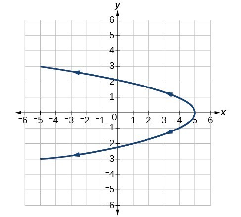
For the following exercises, look at the graphs that were created by parametric equations of the form [latex]\begin{cases}x\left(t\right)=a\text{cos}\left(bt\right)\hfill \\ y\left(t\right)=c\text{sin}\left(dt\right)\hfill \end{cases}[/latex]. Use the parametric mode on the graphing calculator to find the values of [latex]a,b,c[/latex], and [latex]d[/latex] to achieve each graph.
97.
98.
99.
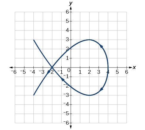
100.
For the following exercises, use a graphing utility to graph the given parametric equations.
- [latex]\begin{cases}x\left(t\right)=\cos t - 1\\ y\left(t\right)=\sin t+t\end{cases}[/latex]
- [latex]\begin{cases}x\left(t\right)=\cos t+t\\ y\left(t\right)=\sin t - 1\end{cases}[/latex]
- [latex]\begin{cases}x\left(t\right)=t-\sin t\\ y\left(t\right)=\cos t - 1\end{cases}[/latex]
101. Graph all three sets of parametric equations on the domain [latex]\left[0,2\pi \right][/latex].
102. Graph all three sets of parametric equations on the domain [latex]\left[0,4\pi \right][/latex].
103. Graph all three sets of parametric equations on the domain [latex]\left[-4\pi ,6\pi \right][/latex].
104. The graph of each set of parametric equations appears to “creep” along one of the axes. What controls which axis the graph creeps along?
105. Explain the effect on the graph of the parametric equation when we switched [latex]\sin t[/latex] and [latex]\cos t[/latex].
106. Explain the effect on the graph of the parametric equation when we changed the domain.
Candela Citations
- Precalculus. Authored by: OpenStax College. Provided by: OpenStax. Located at: http://cnx.org/contents/fd53eae1-fa23-47c7-bb1b-972349835c3c@5.175:1/Preface. License: CC BY: Attribution