(12.1.1) -Define and Evaluate Exponential Functions

India is the second most populous country in the world with a population of about 1.25 billion people in 2013. The population is growing at a rate of about 1.2% each year.^[1] If this rate continues, the population of India will exceed China’s population by the year 2031. When populations grow rapidly, we often say that the growth is “exponential,” meaning that something is increasing very quickly. To a mathematician, however, the term exponential growth has a very specific meaning. In this section, we will take a look at exponential functions, which model this kind of rapid growth.

Linear functions have a constant rate of change – a constant number that the output increases for each increase in input. For example, in the equation [latex]f(x)=3x+4[/latex] , the slope tells us the output increases by three each time the input increases by one. Sometimes, on the other hand, quantities grow by a percent rate of change rather than by a fixed amount. In this lesson, we will define a function whose rate of change increases by a percent of the current value rather than a fixed quantity.

To illustrate this difference consider two companies whose business is expanding: Company A has 100 stores, and expands by opening 50 new stores a year Company B has 100 stores, and expands by increasing the number of stores by 50% of their total each year.

The table below compares the growth of each company where company A increases the number of stores linearly, and company B increases the number of stores by a rate of 50% each year.

Company A has 100 stores and expands by opening 50 new stores a year, so its growth can be represented by the function [latex]A\left(x\right)=100+50x[/latex]. Company B has 100 stores and expands by increasing the number of stores by 50% each year, so its growth can be represented by the function [latex]B\left(x\right)=100{\left(1+0.5\right)}^{x}[/latex].

The graphs comparing the number of stores for each company over a five-year period are shown in below. We can see that, with exponential growth, the number of stores increases much more rapidly than with linear growth.

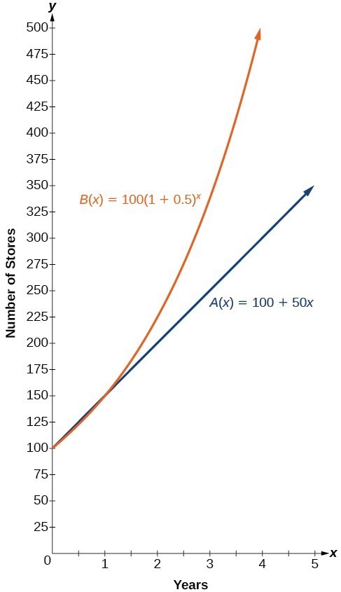
The graph shows the numbers of stores Companies A and B opened over a five-year period.

Notice that the domain for both functions is [latex]\left[0,\infty \right)[/latex], and the range for both functions is [latex]\left[100,\infty \right)[/latex]. After year 1, Company B always has more stores than Company A.

Consider the function representing the number of stores for Company B

[latex]B\left(x\right)=100{\left(1+0.5\right)}^{x}[/latex]

In this exponential function, 100 represents the initial number of stores, 0.50 represents the growth rate, and [latex]1+0.5=1.5[/latex] represents the growth factor. Generalizing further, we can write this function as [latex]B\left(x\right)=100{\left(1.5\right)}^{x}[/latex], where 100 is the initial value, 1.5 is called the base, and [latex]x[/latex] is called the exponent. This is an exponential function.

To evaluate an exponential function with the form [latex]f\left(x\right)={b}^{x}[/latex], we simply substitute x with the given value, and calculate the resulting power. For example:

Let [latex]f\left(x\right)={2}^{x}[/latex]. What is [latex]f\left(3\right)[/latex]?

To evaluate an exponential function with a form other than the basic form, it is important to follow the order of operations. For example:

Let [latex]f\left(x\right)=30{\left(2\right)}^{x}[/latex]. What is [latex]f\left(3\right)[/latex]?

Note that if the order of operations were not followed, the result would be incorrect:

In our first example we will evaluate an exponential function without the aid of a calculator.

In the following video we present more examples of evaluating an exponential function at several different values.

In the next example we will revisit the population of India.

In the following video we show another example of using an exponential function to predict the population of a small town.

(12.1.2) – Define and evaluate a compound interest formula

You may have seen formulas that are used to calculate compound interest rates.  These formulas are another example of exponential growth. The term compounding refers to interest earned not only on the original value, but on the accumulated value of the account. The annual percentage rate (APR) of an account, also called the nominal rate, is the yearly interest rate earned by an investment account.

The term nominal is used when the compounding occurs a number of times other than once per year. In fact, when interest is compounded more than once a year, the effective interest rate ends up being greater than the nominal rate! This is a powerful tool for investing.

We can calculate the compound interest using the compound interest formula, which is an exponential function of the variables time [latex]t[/latex], principal [latex]P[/latex], APR [latex]r[/latex], and number of compounding periods in a year [latex]n[/latex]:

[latex]\displaystyle A\left(t\right)=P{\left(1+\frac{r}{n}\right)}^{nt}[/latex]

In our next example we will calculate the value of an account after 10 years of interest compounded quarterly.

The following video shows an example of using an exponential growth to calculate interest compounded quarterly.

In our next example we will use the compound interest formula to solve for the principal.

In the following video we show another example of finding the deposit amount necessary to obtain a future value from compounded interest.

Define continuous growth as an exponential function with base [latex]e[/latex]

So far we have worked with rational bases for exponential functions. For most real-world phenomena, however, e is used as the base for exponential functions. Exponential models that use e as the base are called continuous growth or decay models. We see these models in finance, computer science, and most of the sciences, such as physics, toxicology, and fluid dynamics.

The Continuous Growth/Decay Formula

For all real numbers [latex]r[/latex], [latex]t[/latex], and all positive numbers [latex]a[/latex], continuous growth or decay is represented by the formula

[latex]A\left(t\right)=a{e}^{rt}[/latex]

where

• [latex]a[/latex] is the initial value,
• [latex]r[/latex] is the continuous growth or decay rate per unit time,
• and [latex]t[/latex] is the elapsed time.

If [latex]r>0[/latex], then the formula represents continuous growth. If [latex]r<0[/latex], then the formula represents continuous decay.

For business applications, the continuous growth formula is called the continuous compounding formula and takes the form

[latex]A\left(t\right)=P{e}^{rt}[/latex]

where

• [latex]P[/latex] is the principal or the initial invested,
• [latex]r[/latex] is the growth or interest rate per unit time,
• and [latex]t[/latex] is the period or term of the investment.

In our next example we will calculate continuous growth of an investment. It is important to note the language that is used in the instructions for interest rate problems.  You will know to use the continuous growth or decay formula when you are asked to find an amount based on continuous compounding.  In previous examples we asked that you find an amount based on quarterly or monthly compounding, and for this you used the compound interest formula.

Example

A person invested $1,000 in an account earning a nominal 10% per year compounded continuously. How much was in the account at the end of one year?

Show Answer

Since the account is growing in value, this is a continuous compounding problem with growth rate [latex]r=0.10[/latex]. The initial investment was $1,000, so [latex]P=1000[/latex]. We use the continuous compounding formula to find the value after [latex]t=1[/latex] year:

[latex]\begin{array}{c}A\left(t\right)\hfill & =P{e}^{rt}\hfill & \text{Use the continuous compounding formula}.\hfill \\ \hfill & =1000{\left(e\right)}^{0.1} & \text{Substitute known values for }P, r,\text{ and }t.\hfill \\ \hfill & \approx 1105.17\hfill & \text{Use a calculator to approximate}.\hfill \end{array}[/latex]

The account is worth $1,105.17 after one year.

In the following video we show another example of continuous interest.

 (12.1.4) – Graph Exponential Functions

We learn a lot about things by seeing their pictorial representations, and that is exactly why graphing exponential equations is a powerful tool. It gives us another layer of insight for predicting future events. Before we begin graphing, it is helpful to review the behavior of exponential growth. Recall the table of values for a function of the form [latex]f\left(x\right)={b}^{x}[/latex] whose base is greater than one. We’ll use the function [latex]f\left(x\right)={2}^{x}[/latex]. Observe how the output values in the table below change as the input increases by 1.

x	–3	–2	–1	0	1	2	3
[latex]f\left(x\right)={2}^{x}[/latex]	[latex]\displaystyle \frac{1}{8}[/latex]	[latex]\displaystyle \frac{1}{4}[/latex]	[latex]\displaystyle \frac{1}{2}[/latex]	1	2	4	8

Each output value is the product of the previous output and the base, 2. We call the base 2 the constant ratio. In fact, for any exponential function with the form [latex]f\left(x\right)=a{b}^{x}[/latex], [latex]b[/latex] is the constant ratio of the function. This means that as the input increases by 1, the output value will be the product of the base and the previous output, regardless of the value of [latex]a[/latex].

Notice from the table that

• the output values are positive for all values of [latex]x[/latex];
• as [latex]x[/latex] increases, the output values increase without bound; and
• as [latex]x[/latex] decreases, the output values grow smaller, approaching zero.

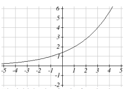
Figure 1 shows the exponential growth function [latex]f\left(x\right)={2}^{x}[/latex].

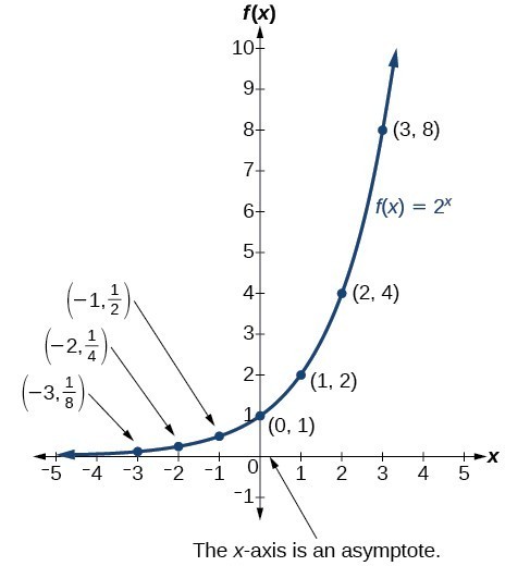
Notice that the graph gets close to the x-axis, but never touches it.

The domain of [latex]f\left(x\right)={2}^{x}[/latex] is all real numbers, the range is [latex]\left(0,\infty \right)[/latex].

To get a sense of the behavior of exponential decay, we can create a table of values for a function of the form [latex]f\left(x\right)={b}^{x}[/latex] whose base is between zero and one. We’ll use the function [latex]\displaystyle g\left(x\right)={\left(\frac{1}{2}\right)}^{x}[/latex]. Observe how the output values in the table below change as the input increases by 1.

x	–3	–2	–1	0	1	2	3
[latex]\displaystyle g\left(x\right)=\left(\frac{1}{2}\right)^{x}[/latex]	8	4	2	1	[latex]\displaystyle \frac{1}{2}[/latex]	[latex]\displaystyle \frac{1}{4}[/latex]	[latex]\displaystyle \frac{1}{8}[/latex]

Again, because the input is increasing by 1, each output value is the product of the previous output and the base, or constant ratio [latex]\displaystyle \frac{1}{2}[/latex].

Notice from the table that

• the output values are positive for all values of [latex]x[/latex];
• as [latex]x[/latex] increases, the output values grow smaller, approaching zero; and
• as [latex]x[/latex] decreases, the output values grow without bound.

The graph shows the exponential decay function, [latex]\displaystyle g\left(x\right)={\left(\frac{1}{2}\right)}^{x}[/latex].

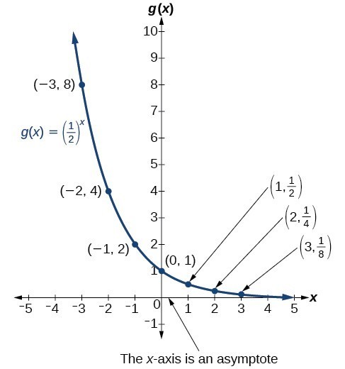
 The domain of [latex]\displaystyle g\left(x\right)={\left(\frac{1}{2}\right)}^{x}[/latex] is all real numbers, the range is [latex]\left(0,\infty \right)[/latex]

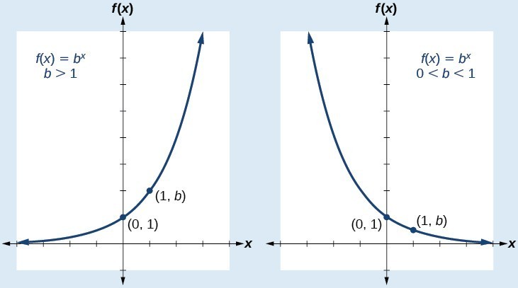
Characteristics of the Graph of  [latex]f(x)=b^x[/latex]

An exponential function with the form [latex]f\left(x\right)={b}^{x}[/latex], [latex]b>0[/latex], [latex]b\ne 1[/latex], has these characteristics:

• one-to-one function
• domain: [latex]\left(-\infty , \infty \right)[/latex]
• range: [latex]\left(0,\infty \right)[/latex]
• [latex]x[/latex]-intercept: none
• [latex]y[/latex]-intercept: [latex]\left(0,1\right)[/latex]
• increasing if [latex]b>1[/latex]
• decreasing if [latex]b<1[/latex]

Compare the graphs of exponential growth and decay functions.

In our first example we will plot an exponential decay function where the base is between 0 and 1.

Example

Sketch a graph of [latex]f\left(x\right)={0.25}^{x}[/latex]. State the domain, range.

Show Answer

Before graphing, identify the behavior and create a table of points for the graph.

• Since [latex]b=0.25[/latex] is between zero and one, we know the function is decreasing, and we can verify this by creating a table of values. The left tail of the graph will increase without bound and the right tail will get really close to the x-axis.
• Create a table of points.
  

  x	–3	–2	–1	0	1	2	3
  [latex]f\left(x\right)={0.25}^{x}[/latex]	64	16	4	1	0.25	0.0625	0.015625

• Plot the y-intercept, [latex]\left(0,1\right)[/latex], along with two other points. We can use [latex]\left(-1,4\right)[/latex] and [latex]\left(1,0.25\right)[/latex].

Draw a smooth curve connecting the points.

 The domain is [latex]\left(-\infty ,\infty \right)[/latex]; the range is [latex]\left(0,\infty \right)[/latex].

In the following video we show another example of graphing an exponential function. The base of the exponential term is between 0 and 1, so this graph will represent decay.

How To: Given an exponential function of the form [latex]f\left(x\right)={b}^{x}[/latex], graph the function.

1. Create a table of points.
2. Plot at least 3 point from the table, including the y-intercept [latex]\left(0,1\right)[/latex].
3. Draw a smooth curve through the points.
4. State the domain, [latex]\left(-\infty ,\infty \right)[/latex], the range, [latex]\left(0,\infty \right)[/latex].

In our next example we will plot an exponential growth function where the base is greater than 1.

Example

Sketch a graph of [latex]f(x)={\sqrt{2}(\sqrt{2})}^{x}[/latex]. State the domain, range.

Show Answer

Before graphing, identify the behavior and create a table of points for the graph.

• Since [latex]b=\sqrt{2}[/latex] which is greater than one, we know the function is increasing, and we can verify this by creating a table of values. The left tail of the graph will get really close to the [latex]x[/latex]-axis and the right tail will increase without bound.
• Create a table of points.
  

  x	–3	–2	–1	0	1	2	3
  [latex]f\left(x\right)=\sqrt{2}{(\sqrt{2})}^{x}[/latex]	0.5	0.71	1	1.41	2	2.83	4

• Plot the [latex]y[/latex]-intercept, [latex]\left(0,1.41\right)[/latex], along with two other points. We can use [latex]\left(-1,1\right)[/latex] and [latex]\left(1,2\right)[/latex].

Draw a smooth curve connecting the points.

The domain is [latex]\left(-\infty ,\infty \right)[/latex]; the range is [latex]\left(0,\infty \right)[/latex].

Our next video example includes graphing an exponential growth function and defining the domain and range of the function.

Summary

Exponential growth grows by a rate proportional to the current amount. For any real number [latex]x[/latex] and any positive real numbers [latex]a[/latex] and [latex]b[/latex] such that [latex]b\ne 1[/latex], an exponential growth function has the form [latex]f\left(x\right)=a{b}^{x}[/latex].  Evaluating exponential functions requires careful attention to the order of operations. Compound interest is an example of exponential growth.

Continuous growth or decay functions are of the form [latex]A\left(t\right)=a{e}^{rt}[/latex]. If [latex]r>0[/latex], then the formula represents continuous growth. If [latex]r<0[/latex], then the formula represents continuous decay. For business applications, the continuous growth formula is called the continuous compounding formula and takes the form [latex]A\left(t\right)=P{e}^{rt}[/latex].

Graphs of exponential growth functions will have a right tail that increases without bound, and a left tail that gets really close to the [latex]x[/latex]-axis. On the other hand, graph so exponential decay functions will have a left tail that increases without bound and a right tail that gets really close to the [latex]x[/latex]-axis. Points can be generated with a table of values and plotted on a set of cartesian axes.