Learning Objectives

(12.3.1) – Define logarithmic functions
- Convert between logarithmic and exponential forms
(12.3.2) – Evaluate Logarithms
- Evaluate logarithms without a calculator
- Define and evaluate natural logarithm
- Define and evaluate common logarithm
(12.3.3) – Graph logarithmic functions
- Identify the domain of a logarithmic function

Photo of the aftermath of the earthquake in Japan with a focus on the Japanese flag.

Figure 1. Devastation of March 11, 2011 earthquake in Honshu, Japan. (credit: Daniel Pierce)

In 2010, a major earthquake struck Haiti, destroying or damaging over 285,000 homes.^[1] One year later, another, stronger earthquake devastated Honshu, Japan, destroying or damaging over 332,000 buildings,^[2] like those shown in the picture above. Even though both caused substantial damage, the earthquake in 2011 was 100 times stronger than the earthquake in Haiti. How do we know? The magnitudes of earthquakes are measured on a scale known as the Richter Scale. The Haitian earthquake registered a 7.0 on the Richter Scale^[3] whereas the Japanese earthquake registered a 9.0.^[4]

The Richter Scale is a base-ten logarithmic scale. In other words, an earthquake of magnitude 8 is not twice as great as an earthquake of magnitude 4. It is ${10}^{8 - 4}={10}^{4}=10,000$ times as great! In this lesson, we will investigate the nature of the Richter Scale and the base-ten function upon which it depends.

In the last section, we defined inverse functions, logarithmic functions are the inverse of an exponential functions, and sometimes understanding this helps us make sense of what a logarithm is.

(12.3.1) – Define Logarithmic Functions

In order to analyze the magnitude of earthquakes or compare the magnitudes of two different earthquakes, we need to be able to convert between logarithmic and exponential form. For example, suppose the amount of energy released from one earthquake were 500 times greater than the amount of energy released from another. We want to calculate the difference in magnitude. The equation that represents this problem is ${10}^{x}=500$ , where $x$ represents the difference in magnitudes on the Richter Scale. How would we solve for $x$ ?

We have not yet learned a method for solving exponential equations. None of the algebraic tools discussed so far is sufficient to solve ${10}^{x}=500$ . We know that ${10}^{2}=100$ and ${10}^{3}=1000$ , so it is clear that $x$ must be some value between 2 and 3, since $y={10}^{x}$ is increasing. We can examine a graph to better estimate the solution.

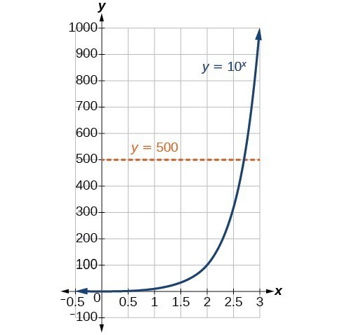
Graph of the intersections of the equations y=10^x and y=500.

Figure 2

Estimating from a graph, however, is imprecise. To find an algebraic solution, we must introduce a new function. Observe that the graph above passes the horizontal line test. The exponential function $y={b}^{x}$ is one-to-one, so its inverse, $x={b}^{y}$ is also a function. As is the case with all inverse functions, we simply interchange $x$ and $y$ and solve for $y$ to find the inverse function. To represent $y$ as a function of $x$ , we use a logarithmic function of the form $y={\mathrm{log}}_{b}\left(x\right)$ . The base $b$ logarithm of a number is the exponent by which we must raise $b$ to get that number.

We read a logarithmic expression as, “The logarithm with base $b$ of $x$ is equal to $y$ ,” or, simplified, “log base $b$ of $x$ is $y$ .” We can also say, “ $b$ raised to the power of $y$ is $x$ ,” because logs are exponents. For example, the base 2 logarithm of 32 is 5, because 5 is the exponent we must apply to 2 to get 32. Since ${2}^{5}=32$ , we can write ${\mathrm{log}}_{2}32=5$ . We read this as “log base 2 of 32 is 5.”

We can express the relationship between logarithmic form and its corresponding exponential form as follows:

{l o g}_{b} (x) = y \Leftrightarrow b^{y} = x, b > 0, b \neq 1

${\mathrm{log}}_{b}\left(x\right)=y\Leftrightarrow {b}^{y}=x,\text{}b>0,b\ne 1$

Note that the base $b$ is always positive.
Think b to the y equals x.

Because logarithm is a function, it is most correctly written as ${\mathrm{log}}_{b}\left(x\right)$ , using parentheses to denote function evaluation, just as we would with $f\left(x\right)$ . However, when the input is a single variable or number, it is common to see the parentheses dropped and the expression written without parentheses, as ${\mathrm{log}}_{b}x$ . Note that many calculators require parentheses around the $x$ .

We can illustrate the notation of logarithms as follows:
logb (c) = a means b to the A power equals C.

Notice that, comparing the logarithm function and the exponential function, the input and the output are switched. This means $y={\mathrm{log}}_{b}\left(x\right)$ and $y={b}^{x}$ are inverse functions.

Definition of the Logarithmic Function

A logarithm base $b$ of a positive number $x$ satisfies the following definition.

For $x>0,b>0,b\ne 1$ ,

y = {l o g}_{b} (x) is equivalent to b^{y} = x

$y={\mathrm{log}}_{b}\left(x\right)\text{ is equivalent to }{b}^{y}=x$

where,

we read ${\mathrm{log}}_{b}\left(x\right)$ as, “the logarithm with base $b$ of $x$ ” or the “log base $b$ of $x$ .”
the logarithm $y$ is the exponent to which $b$ must be raised to get $x$ .

Also, since the logarithmic and exponential functions switch the $x$ and $y$ values, the domain and range of the exponential function are interchanged for the logarithmic function. Therefore,

the domain of the logarithm function with base $b \text{ is} \left(0,\infty \right)$ .
the range of the logarithm function with base $b \text{ is} \left(-\infty ,\infty \right)$ .

Convert between logarithmic and exponential forms

In our first example we will convert logarithmic equations into exponential equations.

Example

Write the following logarithmic equations in exponential form.

${\mathrm{log}}_{6}\left(\sqrt{6}\right)=\frac{1}{2}$
log3(9)=2 ${l o g}_{3} (9) = 2$
Show Answer
First, identify the values of $b$ , $y$ , and $x$ . Then, write the equation in the form ${b}^{y}=x$ .
1. $\displaystyle {\mathrm{log}}_{6}\left(\sqrt{6}\right)=\frac{1}{2}$
  Here, $b=6,y=\frac{1}{2},\text{and } x=\sqrt{6}$ . Therefore, the equation $\displaystyle {\mathrm{log}}_{6}\left(\sqrt{6}\right)=\frac{1}{2}$ is equivalent to $\displaystyle {6}^{\frac{1}{2}}=\sqrt{6}$ .
2. ${\mathrm{log}}_{3}\left(9\right)=2$
  Here, $b=3$ , $y=2$ , and $x=9$ . Therefore, the equation ${\mathrm{log}}_{3}\left(9\right)=2$ is equivalent to ${3}^{2}=9$ .

In the following video we present more examples of rewriting logarithmic equations as exponential equations.

How To: Given an equation in logarithmic form ${\mathrm{log}}_{b}\left(x\right)=y$ , convert it to exponential form.

Examine the equation $y={\mathrm{log}}_{b}x$ and identify $b$ , $y$ , and $x$ .
Rewrite ${\mathrm{log}}_{b}x=y$ as ${b}^{y}=x$ .

Think About It

Can we take the logarithm of a negative number? Re-read the definition of a logarithm and formulate an answer. Think about the behavior of exponents. You can use the textbox below to formulate your ideas before you look at an answer.

Show Answer

Convert from exponential to logarithmic form

To convert from exponents to logarithms, we follow the same steps in reverse. We identify the base $b$ , exponent $x$ , and output $y$ . Then we write $x={\mathrm{log}}_{b}\left(y\right)$ .

Example

Write the following exponential equations in logarithmic form.

${2}^{3}=8$
${5}^{2}=25$
10−4=110,000 $10^{- 4} = \frac{1}{10, 000}$
Show Answer
First, identify the values of $b$ , $y$ , and $x$ . Then, write the equation in the form $x={\mathrm{log}}_{b}\left(y\right)$ .
1. ${2}^{3}=8$
  Here, $b=2$ , $x=3$ , and $y=8$ . Therefore, the equation ${2}^{3}=8$ is equivalent to ${\mathrm{log}}_{2}\left(8\right)=3$ .
2. ${5}^{2}=25$
  Here, $b=5$ , $x=2$ , and $y=25$ . Therefore, the equation ${5}^{2}=25$ is equivalent to ${\mathrm{log}}_{5}\left(25\right)=2$ .
3. $\displaystyle {10}^{-4}=\frac{1}{10,000}$
  Here, $b=10$ , $x=-4$ , and $\displaystyle y=\frac{1}{10,000}$ . Therefore, the equation $\displaystyle {10}^{-4}=\frac{1}{10,000}$ is equivalent to $\displaystyle {\text{log}}_{10}\left(\frac{1}{10,000}\right)=-4$ .

In the next video we show more examples of writing logarithmic equations as exponential equations.

(12.3.2) – Evaluate Logarithms

Knowing the squares, cubes, and roots of numbers allows us to evaluate many logarithms mentally. For example, consider ${\mathrm{log}}_{2}8$ . We ask, “To what exponent must 2 be raised in order to get 8?” Because we already know ${2}^{3}=8$ , it follows that ${\mathrm{log}}_{2}8=3$ .

Now consider solving ${\mathrm{log}}_{7}49$ and ${\mathrm{log}}_{3}27$ mentally.

We ask, “To what exponent must 7 be raised in order to get 49?” We know ${7}^{2}=49$ . Therefore, ${\mathrm{log}}_{7}49=2$
We ask, “To what exponent must 3 be raised in order to get 27?” We know ${3}^{3}=27$ . Therefore, ${\mathrm{log}}_{3}27=3$

Even some seemingly more complicated logarithms can be evaluated without a calculator. For example, let’s evaluate $\displaystyle {\mathrm{log}}_{\frac{2}{3}}\frac{4}{9}$ mentally.

We ask, “To what exponent must $\frac{2}{3}$ be raised in order to get $\displaystyle \frac{4}{9}$ ? ” We know ${2}^{2}=4$ and ${3}^{2}=9$ , so $\displaystyle {\left(\frac{2}{3}\right)}^{2}=\frac{4}{9}$ . Therefore, $\displaystyle {\mathrm{log}}_{\frac{2}{3}}\left(\frac{4}{9}\right)=2$ .

In our first example we will evaluate logarithms mentally (without a calculator).

Example

Solve $y={\mathrm{log}}_{4}\left(64\right)$ without using a calculator.

Show Answer

First we rewrite the logarithm in exponential form: ${4}^{y}=64$ . Next, we ask, “To what exponent must 4 be raised in order to get 64?”

We know

4^{3} = 64

${4}^{3}=64$

Therefore,

l o g_{4} (64) = 3

$\mathrm{log}{}_{4}\left(64\right)=3$

In our first video we will show more examples of evaluating logarithms mentally, this helps you get familiar with what a logarithm represents.

In our next example we will evaluate the logarithm of a reciprocal.

Example

Evaluate $y={\mathrm{log}}_{3}\left(\frac{1}{27}\right)$ without using a calculator.

Show Answer

First we rewrite the logarithm in exponential form: $\displaystyle {3}^{y}=\frac{1}{27}$ . Next, we ask, “To what exponent must 3 be raised in order to get $\frac{1}{27}$ “?

We know ${3}^{3}=27$ , but what must we do to get the reciprocal, $\displaystyle \frac{1}{27}$ ? Recall from working with exponents that $\displaystyle {b}^{-a}=\frac{1}{{b}^{a}}$ . We use this information to write

\begin{matrix} 3^{- 3} & = & \frac{1}{3^{3}} = & \frac{1}{27} \end{matrix}

$\large \begin{array}{c} {3}^{-3}&=&\frac{1}{{3}^{3}}\hfill \\ &=&\frac{1}{27}\hfill \end{array}$

Therefore, $\displaystyle {\mathrm{log}}_{3}\left(\frac{1}{27}\right)=-3$ .

How To: Given a logarithm of the form $y={\mathrm{log}}_{b}\left(x\right)$ , evaluate it without a calculator.

Rewrite the argument $x$ as a power of $b$ : ${b}^{y}=x$ .
Use previous knowledge of powers of $b$ identify $y$ by asking, “To what exponent should $b$ be raised in order to get $x$ ?”

Define and evaluate natural logarithm

The most frequently used base for logarithms is [latex]e[/latex]. Base [latex]e[/latex] logarithms are important in calculus and some scientific applications; they are called natural logarithms. The base e logarithm, ${\mathrm{log}}_{e}\left(x\right)$ , has its own notation, $\mathrm{ln}\left(x\right)$ .

Most values of $\mathrm{ln}\left(x\right)$ can be found only using a calculator. The major exception is that, because the logarithm of 1 is always 0 in any base, $\mathrm{ln}1=0$ . For other natural logarithms, we can use the $\mathrm{ln}$ key that can be found on most scientific calculators. We can also find the natural logarithm of any power of e using the inverse property of logarithms.

A General Note: Definition of the Natural Logarithm

A natural logarithm is a logarithm with base e. We write ${\mathrm{log}}_{e}\left(x\right)$ simply as $\mathrm{ln}\left(x\right)$ . The natural logarithm of a positive number $x$ satisfies the following definition.

For $x>0$ ,

y = l n (x) is equivalent to e^{y} = x

$y=\mathrm{ln}\left(x\right)\text{ is equivalent to }{e}^{y}=x$

We read $\mathrm{ln}\left(x\right)$ as, “the logarithm with base $e$ of $x$ ” or “the natural logarithm of $x$ .”

The logarithm $y$ is the exponent to which $e$ must be raised to get $x$ .

Since the functions $y=e{}^{x}$ and $y=\mathrm{ln}\left(x\right)$ are inverse functions, $\mathrm{ln}\left({e}^{x}\right)=x$ for all $x$ and $e{}^{\mathrm{ln}\left(x\right)}=x$ for $x>0$ .

In the next example, we will evaluate a natural logarithm using a calculator.

Example

Evaluate $y=\mathrm{ln}\left(500\right)$ to four decimal places using a calculator.

Show Answer

Press [LN].
Enter 500, followed by [ ) ].
Press [ENTER].

Rounding to four decimal places, $\mathrm{ln}\left(500\right)\approx 6.2146$

In our next video, we show more examples of how to evaluate natural logarithms using a calculator.

Define and evaluate common logarithm

Sometimes we may see a logarithm written without a base. In this case, we assume that the base is 10. In other words, the expression ${\mathrm{log}}_{}$ means ${\mathrm{log}}_{10}$ We call a base-10 logarithm a common logarithm. Common logarithms are used to measure the Richter Scale mentioned at the beginning of the section. Scales for measuring the brightness of stars and the pH of acids and bases also use common logarithms.

Definition of Common Logarithm: Log is an exponent

A common logarithm is a logarithm with base 10. We write ${\mathrm{log}}_{10}(x)$ simplify as ${\mathrm{log}}_{}(x)$ . The common logarithm of a positive number, $x$ , satisfies the following definition:

For $x\gt0$

$y={\mathrm{log}}_{}(x)$ is equivalent to $10^y=x$

We read ${\mathrm{log}}_{}(x)$ as ” the logarithm with base 10 of $x$ ” or “log base 10 of $x$ “.

The logarithm y is the exponent to which 10 must be raised to get $x$ .

Example

Evaluate ${\mathrm{log}}_{}(1000)$ without using a calculator.

Show Answer

We know $10^3=1000$ , therefore ${\mathrm{log}}_{}(1000)=3$

Example

Evaluate $y={\mathrm{log}}_{}(321)$ to four decimal places using a calculator.

Show Answer

Press [LOG].
Enter 321, followed by [ ) ].
Press [ENTER].

Rounding to four decimal places, ${\mathrm{log}}_{}(321)\approx2.5065$

In our last example we will use a logarithm to find the difference in magnitude of two different earthquakes.

Example

The amount of energy released from one earthquake was 500 times greater than the amount of energy released from another. The equation $10^x=500$ represents this situation, where $x$ is the difference in magnitudes on the Richter Scale. To the nearest thousandth, what was the difference in magnitudes?

Show Answer

We begin by rewriting the exponential equation in logarithmic form.

$10^x=500$

${\mathrm{log}}_{}(500)=x$

Next we evaluate the logarithm using a calculator:

Press [LOG].
Enter 500 followed by [ ) ].
Press [ENTER].
To the nearest thousandth, ${\mathrm{log}}_{}(500)\approx2.699$ $y = {l o g}_{b} (x)$

(12.3.3) – Graph Logarithmic Functions

Before working with graphs, we will take a look at the domain (the set of input values) for which the logarithmic function is defined.

Recall that the exponential function is defined as $y={b}^{x}$ for any real number x and constant $b>0$ , $b\ne 1$ , where

The domain of $x$ is $\left(-\infty ,\infty \right)$ .
The range of $y$ is $\left(0,\infty \right)$ .

In the last section we learned that the logarithmic function $y={\mathrm{log}}_{b}\left(x\right)$ is the inverse of the exponential function $y={b}^{x}$ . So, as inverse functions:

The domain of $y={\mathrm{log}}_{b}\left(x\right)$ is the range of $y={b}^{x}$ : $\left(0,\infty \right)$ .
The range of $y={\mathrm{log}}_{b}\left(x\right)$ is the domain of $y={b}^{x}$ : $\left(-\infty ,\infty \right)$ .

How To: Given a logarithmic function, identify the domain.

Set up an inequality showing the argument greater than zero.
Solve for $x$ .
Write the domain in interval notation.

In our first example we will show how to identify the domain of a logarithmic function.

Example

What is the domain of $f(x)={\mathrm{log}}_{2}\left(x+3\right)$ ?

Show Answer

The logarithmic function is defined only when the input is positive, so this function is defined when $x+3>0$ . Solving this inequality,

\begin{matrix} x + 3 > 0 & The input must be positive . x > - 3 & Subtract 3 . \end{matrix}

$\begin{array}{c}x+3>0\hfill & \text{The input must be positive}.\hfill \\ x>-3\hfill & \text{Subtract 3}.\hfill \end{array}$

The domain of $f\left(x\right)={\mathrm{log}}_{2}\left(x+3\right)$ is $\left(-3,\infty \right)$ .

Here is another example of how to identify the domain of a logarithmic function.

Example

What is the domain of $f\left(x\right)=\mathrm{log}\left(5 - 2x\right)$ ?

Show Answer

The logarithmic function is defined only when the input is positive, so this function is defined when $5 - 2x>0$ . Solving this inequality,

\begin{matrix} 5 - 2 x & > & 0 & The input must be positive . - 2 x & > & - 5 & Subtract 5. x & < & \frac{5}{2} & Divide by - 2 and switch the inequality . \end{matrix}

$\begin{array}{c}5 - 2x&>&0\hfill & \text{The input must be positive}.\hfill \\ -2x&>&-5\hfill & \text{Subtract }5.\hfill \\ x&<& \displaystyle \frac{5}{2}& \text{Divide by }-2\text{ and switch the inequality}.\hfill \end{array}$

The domain of $f\left(x\right)=\mathrm{log}\left(5 - 2x\right)$ is $\displaystyle \left(-\infty ,\frac{5}{2}\right)$ .

Creating a graphical representation of most functions gives us another layer of insight for predicting future events. How do logarithmic graphs give us insight into situations? Because every logarithmic function is the inverse function of an exponential function, we can think of every output on a logarithmic graph as the input for the corresponding inverse exponential equation. In other words, logarithms give the cause for an effect.

To illustrate, suppose we invest $2500 in an account that offers an annual interest rate of 5%, compounded continuously. We already know that the balance in our account for any year t can be found with the equation $A=2500{e}^{0.05t}$ .

But what if we wanted to know the year for any balance? We would need to create a corresponding new function by interchanging the input and the output; thus we would need to create a logarithmic model for this situation. By graphing the model, we can see the output (year) for any input (account balance). For instance, what if we wanted to know how many years it would take for our initial investment to double? Figure 1 shows this point on the logarithmic graph.

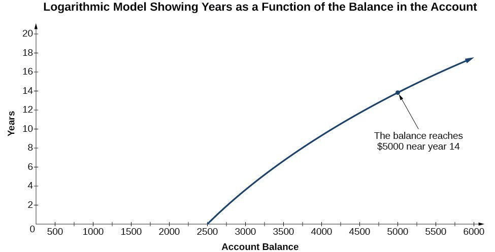
Figure 1

Now that we have a feel for the set of values for which a logarithmic function is defined, we move on to graphing logarithmic functions. The family of logarithmic functions includes the parent function $y={\mathrm{log}}_{b}\left(x\right)$ along with all its transformations: shifts, stretches, compressions, and reflections.

We begin with the parent function $y={\mathrm{log}}_{b}\left(x\right)$ . Because every logarithmic function of this form is the inverse of an exponential function with the form $y={b}^{x}$ , their graphs will be reflections of each other across the line $y=x$ . To illustrate this, we can observe the relationship between the input and output values of $y={2}^{x}$ and its equivalent $x={\mathrm{log}}_{2}\left(y\right)$ in the table below.

x	–3	–2	–1	0	1	2	3
${2}^{x}=y$	$\displaystyle \frac{1}{8}$	$\displaystyle \frac{1}{4}$	$\displaystyle \frac{1}{2}$	1	2	4	8
${\mathrm{log}}_{2}\left(y\right)=x$	–3	–2	–1	0	1	2	3

Using the inputs and outputs from the table above, we can build another table to observe the relationship between points on the graphs of the inverse functions $f\left(x\right)={2}^{x}$ and $g\left(x\right)={\mathrm{log}}_{2}\left(x\right)$ .

$f\left(x\right)={2}^{x}$	$\displaystyle \left(-3,\frac{1}{8}\right)$	$\displaystyle \left(-2,\frac{1}{4}\right)$	$\displaystyle \left(-1,\frac{1}{2}\right)$	$\left(0,1\right)$	$\left(1,2\right)$	$\left(2,4\right)$	$\left(3,8\right)$
$g\left(x\right)={\mathrm{log}}_{2}\left(x\right)$	$\displaystyle \left(\frac{1}{8},-3\right)$	$\displaystyle\left(\frac{1}{4},-2\right)$	$\displaystyle \left(\frac{1}{2},-1\right)$	$\left(1,0\right)$	$\left(2,1\right)$	$\left(4,2\right)$	$\left(8,3\right)$

As we’d expect, the $x$ – and $y$ -coordinates are reversed for the inverse functions. The figure below shows the graph of $f$ and $g$ .

Graph of two functions, f(x)=2^x and g(x)=log_2(x), with the line y=x denoting the axis of symmetry.

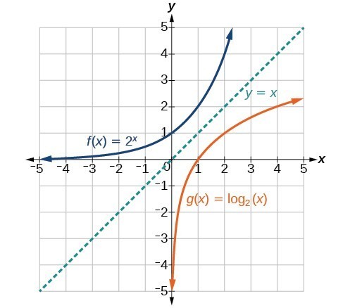
Notice that the graphs of $f\left(x\right)={2}^{x}$ and $g\left(x\right)={\mathrm{log}}_{2}\left(x\right)$ are reflections about the line $y=x$ .

Observe the following from the graph:

$f\left(x\right)={2}^{x}$ has a $y$ -intercept at $\left(0,1\right)$ and $g\left(x\right)={\mathrm{log}}_{2}\left(x\right)$ has an $x$ -intercept at $\left(1,0\right)$ .
The domain of $f\left(x\right)={2}^{x}$ , $\left(-\infty ,\infty \right)$ , is the same as the range of $g\left(x\right)={\mathrm{log}}_{2}\left(x\right)$ .
The range of $f\left(x\right)={2}^{x}$ , $\left(0,\infty \right)$ , is the same as the domain of $g\left(x\right)={\mathrm{log}}_{2}\left(x\right)$ .

A General Note: Characteristics of the Graph $f(x)=\log_b{(x)}$

For any real number $x$ and constant $b>0$ , $b\ne 1$ , we can see the following characteristics in the graph of $f\left(x\right)={\mathrm{log}}_{b}\left(x\right)$ :

domain: $\left(0,\infty \right)$
range: $\left(-\infty ,\infty \right)$
$x$ -intercept: $\left(1,0\right)$ and key point $\left(b,1\right)$
$y$ -intercept: none
increasing if $b>1$
decreasing if [latex]0

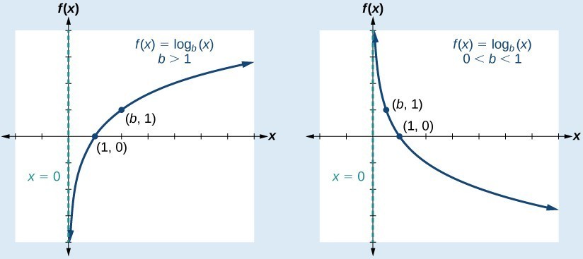
Two graphs of the function f(x)=log_b(x) with points (1,0) and (b, 1). The first graph shows the line when b>1, and the second graph shows the line when 0<b<1.

Figure 3 shows how changing the base $b$ in $f\left(x\right)={\mathrm{log}}_{b}\left(x\right)$ can affect the graphs. Observe that the graphs compress vertically as the value of the base increases. (Note: recall that the function $\mathrm{ln}\left(x\right)$ has base $e\approx \text{2}.\text{718.)}$

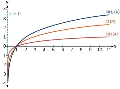
Graph of three equations: y=log_2(x) in blue, y=ln(x) in orange, and y=log(x) in red. The y-axis is the asymptote.

Figure 4. The graphs of three logarithmic functions with different bases, all greater than 1.

In our first example we will graph a logarithmic function of the form $f\left(x\right)={\mathrm{log}}_{b}\left(x\right)$ .

Example

Graph $f\left(x\right)={\mathrm{log}}_{5}\left(x\right)$ . State the domain, range.

Show Answer

Before graphing, identify the behavior and key points for the graph.

Since $b=5$ is greater than one, we know the function is increasing. The left tail of the graph will approach the vertical line $x=0$ , and the right tail will increase slowly without bound.
The $x$ -intercept is $\left(1,0\right)$ .
The key point $\left(5,1\right)$ is on the graph.
We plot and label the points, and draw a smooth curve through the points.

Graph of f(x)=log_5(x) with labeled points at (1, 0) and (5, 1). The y-axis is the asymptote.

Figure 5. The domain is $\left(0,\infty \right)$ , the range is $\left(-\infty ,\infty \right)$ .

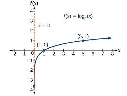
How To: Given a logarithmic function with the form $f\left(x\right)={\mathrm{log}}_{b}\left(x\right)$ , graph the function.

Plot the $x$ -intercept, $\left(1,0\right)$ .
Plot the key point $\left(b,1\right)$ .
Draw a smooth curve through the points.
State the domain, $\left(0,\infty \right)$ , the range, $\left(-\infty ,\infty \right)$ .

Summary

The base $b$ logarithm of a number is the exponent by which we must raise $b$ to get that number. Logarithmic functions are the inverse of Exponential functions, and it is often easier to understand them through this lens. We can never take the logarithm of a negative number, therefore ${\mathrm{log}}_{b}\left(x\right)=y$ is defined for $b>0$ .

Knowing the squares, cubes, and roots of numbers allows us to evaluate many logarithms mentally because the logarithm is an exponent. Logarithms most commonly sue base 10, and often use base e. Logarithms can also be evaluated with most kinds of calculator.

To define the domain of a logarithmic function algebraically, set the argument greater than zero and solve. To plot a logarithmic function, it is easiest to find and plot the $x$ -intercept, and the key point $\left(b,1\right)$ .

http://earthquake.usgs.gov/earthquakes/eqinthenews/2010/us2010rja6/#summary. Accessed 3/4/2013. ↵
http://earthquake.usgs.gov/earthquakes/eqinthenews/2011/usc0001xgp/#summary. Accessed 3/4/2013. ↵
http://earthquake.usgs.gov/earthquakes/eqinthenews/2010/us2010rja6/. Accessed 3/4/2013. ↵
http://earthquake.usgs.gov/earthquakes/eqinthenews/2011/usc0001xgp/#details. Accessed 3/4/2013. ↵

Module 12: Exponential and Logarithmic Functions

12.3 – Logarithmic Functions

Learning Objectives

(12.3.1) – Define Logarithmic Functions

Definition of the Logarithmic Function

Convert between logarithmic and exponential forms

Example

How To: Given an equation in logarithmic form ${\mathrm{log}}_{b}\left(x\right)=y$ , convert it to exponential form.

Think About It

Convert from exponential to logarithmic form

Example

(12.3.2) – Evaluate Logarithms

Example

Example

How To: Given a logarithm of the form $y={\mathrm{log}}_{b}\left(x\right)$ , evaluate it without a calculator.

Define and evaluate natural logarithm

A General Note: Definition of the Natural Logarithm

Example

Define and evaluate common logarithm

Definition of Common Logarithm: Log is an exponent

Example

Example

Example

(12.3.3) – Graph Logarithmic Functions

How To: Given a logarithmic function, identify the domain.

Example

Example

A General Note: Characteristics of the Graph $f(x)=\log_b{(x)}$

Example

How To: Given a logarithmic function with the form $f\left(x\right)={\mathrm{log}}_{b}\left(x\right)$ , graph the function.

Summary

Candela Citations

Module 12: Exponential and Logarithmic Functions

12.3 – Logarithmic Functions

Learning Objectives

(12.3.1) – Define Logarithmic Functions

Definition of the Logarithmic Function

Convert between logarithmic and exponential forms

Example

How To: Given an equation in logarithmic form logb(x)=ylogb(x)=y{\mathrm{log}}_{b}\left(x\right)=y, convert it to exponential form.

Think About It

Convert from exponential to logarithmic form

Example

(12.3.2) – Evaluate Logarithms

Example

Example

How To: Given a logarithm of the form y=logb(x)y=logb(x)y={\mathrm{log}}_{b}\left(x\right), evaluate it without a calculator.

Define and evaluate natural logarithm

A General Note: Definition of the Natural Logarithm

Example

Define and evaluate common logarithm

Definition of Common Logarithm: Log is an exponent

Example

Example

Example

(12.3.3) – Graph Logarithmic Functions

How To: Given a logarithmic function, identify the domain.

Example

Example

A General Note: Characteristics of the Graph f(x)=logb(x)f(x)=\log_b{(x)}

Example

How To: Given a logarithmic function with the form f(x)=logb(x)f\left(x\right)={\mathrm{log}}_{b}\left(x\right), graph the function.

Summary

How To: Given an equation in logarithmic form ${\mathrm{log}}_{b}\left(x\right)=y$ , convert it to exponential form.

How To: Given a logarithm of the form $y={\mathrm{log}}_{b}\left(x\right)$ , evaluate it without a calculator.

A General Note: Characteristics of the Graph $f(x)=\log_b{(x)}$

How To: Given a logarithmic function with the form $f\left(x\right)={\mathrm{log}}_{b}\left(x\right)$ , graph the function.