(6.4.1) – Define solutions to a linear inequality in two variables

Previously we learned to solve inequalities with only one variable. We will now learn about inequalities containing two variables. In particular we will look at linear inequalities in two variables which are very similar to linear equations in two variables.

Linear inequalities in two variables have many applications. If you ran a business, for example, you would want your revenue to be greater than your costs—so that your business made a profit.

Recall that an inequality with one variable had many solutions. For example, the solution to the inequality [latex]x > 3[/latex] is any number greater than 3. We showed this on the number line by shading in the number line to the right of 3, and putting an open parenthesis at 3.

Similarly, linear inequalities in two variables have many solutions. Any ordered pair [latex](x,y)[/latex] that makes an inequality true when we substitute in the values is a solution to a linear inequality.

Solution Sets of Inequalities

The graph below shows the region of values that makes the inequality [latex]3x+2y\leq6[/latex] true (shaded red), the boundary line [latex]3x+2y=6[/latex], as well as a handful of ordered pairs. The boundary line is solid because points on the boundary line [latex]3x+2y=6[/latex] will make the inequality [latex]3x+2y\leq6[/latex] true.

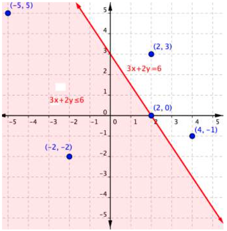
You can substitute the [latex]x[/latex]– and [latex]y[/latex]–values in each of the [latex](x,y)[/latex] ordered pairs into the inequality to find solutions. Sometimes making a table of values makes sense for more complicated inequalities.

If substituting [latex](x,y)[/latex] into the inequality yields a true statement, then the ordered pair is a solution to the inequality, and the point will be plotted within the shaded region or the point will be part of a solid boundary line. A false statement means that the ordered pair is not a solution, and the point will graph outside the shaded region, or the point will be part of a dotted boundary line.

Example

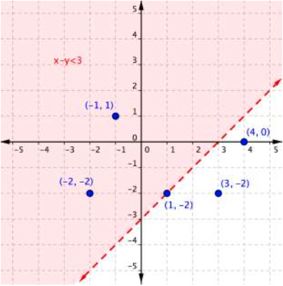
Use the graph to determine which ordered pairs plotted below are solutions of the inequality [latex]x–y<3[/latex].

Show Solution

Solutions will be located in the shaded region. Since this is a “less than” problem, ordered pairs on the boundary line are not included in the solution set.

These values are located in the shaded region, so are solutions. (When substituted into the inequality [latex]x–y<3[/latex], they produce true statements.)

[latex](−1,1)[/latex]

[latex](−2,−2)[/latex]

These values are not located in the shaded region, so are not solutions. (When substituted into the inequality [latex]x-y<3[/latex], they produce false statements.)

[latex](1,−2)[/latex]

[latex](3,−2)[/latex]

[latex](4,0)[/latex]

Answer

[latex](−1,1)\,\,\,(−2,−2)[/latex]

The following video show an example of determining whether an ordered pair is a solution to an inequality.

The following video shows another example of determining whether an ordered pair is a solution to an inequality.

(6.4.2) – Graphing the solution set to a linear inequality in two variables

So how do you get from the algebraic form of an inequality, like [latex]y>3x+1[/latex], to a graph of that inequality? Plotting inequalities is fairly straightforward if you follow a couple steps.

Let’s graph the inequality [latex]x+4y\leq4[/latex].

To graph the boundary line, find at least two values that lie on the line [latex]x+4y=4[/latex]. You can use the x– and y-intercepts for this equation by substituting 0 in for x first and finding the value of y; then substitute 0 in for y and find x.

Plot the points [latex](0,1)[/latex] and [latex](4,0)[/latex], and draw a line through these two points for the boundary line. The line is solid because ≤ means “less than or equal to,” so all ordered pairs along the line are included in the solution set.

The next step is to find the region that contains the solutions. Is it above or below the boundary line? To identify the region where the inequality holds true, you can test a couple of ordered pairs, one on each side of the boundary line.

If you substitute [latex](−1,3)[/latex] into [latex]x+4y\leq4[/latex]:

[latex]\begin{array}{r}−1+4\left(3\right)\leq4\\−1+12\leq4\\11\leq4\end{array}[/latex]

This is a false statement, since 11 is not less than or equal to 4.

On the other hand, if you substitute [latex](2,0)[/latex] into [latex]x+4y\leq4[/latex]:

[latex]\begin{array}{r}2+4\left(0\right)\leq4\\2+0\leq4\\2\leq4\end{array}[/latex]

This is true! The region that includes [latex](2,0)[/latex] should be shaded, as this is the region of solutions.

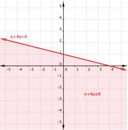
And there you have it—the graph of the set of solutions for [latex]x+4y\leq4[/latex].

Example

Graph the inequality [latex]2y>4x–6[/latex].

Show Solution

Solve for [latex]y[/latex].

[latex] \displaystyle \begin{array}{r}2y>4x-6\\\\\frac{2y}{2}>\frac{4x}{2}-\frac{6}{2}\\\\y>2x-3\\\end{array}[/latex]

Create a table of values to find two points on the line [latex] \displaystyle y=2x-3[/latex], or graph it based on the slope-intercept method, the [latex]b[/latex] value of the [latex]y[/latex]-intercept is [latex]-3[/latex] and the slope is 2.

Plot the points, and graph the line. The line is dotted because the sign in the inequality is >, not ≥ and therefore points on the line are not solutions to the inequality.

[latex] \displaystyle y=2x-3[/latex]

x	y
0	[latex]−3[/latex]
2	1

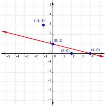
Find an ordered pair on either side of the boundary line. Insert the [latex]x[/latex]– and [latex]y[/latex]-values into the inequality
[latex]2y>4x–6[/latex] and see which ordered pair results in a true statement. Since [latex](−3,1)[/latex] results in a true statement, the region that includes [latex](−3,1)[/latex] should be shaded.

[latex]\begin{array}{l}2y>4x–6\\\\\text{Test }1:\left(−3,1\right)\\2\left(1\right)>4\left(−3\right)–6\\\,\,\,\,\,\,\,2>–12–6\\\,\,\,\,\,\,\,2>−18\\\text{TRUE}\\\\\text{Test }2:\left(4,1\right)\\2(1)>4\left(4\right)– 6\\\,\,\,\,\,\,2>16–6\\\,\,\,\,\,\,2>10\\\text{FALSE}\end{array}[/latex]

Answer

The graph of the inequality [latex]2y>4x–6[/latex] is:

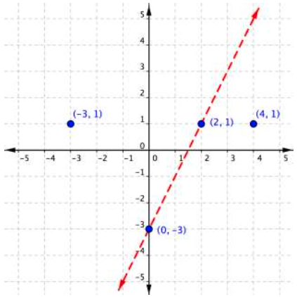
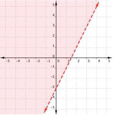
A quick note about the problem above—notice that you can use the points [latex](0,−3)[/latex] and [latex](2,1)[/latex] to graph the boundary line, but that these points are not included in the region of solutions, since the region does not include the boundary line!

(6.4.3) – Graph a system of linear inequalities and define the solutions region

Consider the graph of the inequality [latex]y<2x+5[/latex].

The dashed line is [latex]y=2x+5[/latex]. Every ordered pair in the shaded area below the line is a solution to [latex]y<2x+5[/latex], as all of the points below the line will make the inequality true. If you doubt that, try substituting the [latex]x[/latex] and [latex]y[/latex] coordinates of Points A and B into the inequality—you’ll see that they work. So, the shaded area shows all of the solutions for this inequality.

The boundary line divides the coordinate plane in half. In this case, it is shown as a dashed line as the points on the line don’t satisfy the inequality. If the inequality had been [latex]y\leq2x+5[/latex], then the boundary line would have been solid.

Let’s graph another inequality: [latex]y>−x[/latex]. You can check a couple of points to determine which side of the boundary line to shade. Checking points M and N yield true statements. So, we shade the area above the line. The line is dashed as points on the line are not true.

To create a system of inequalities, you need to graph two or more inequalities together. Let’s use [latex]y<2x+5[/latex] and [latex]y>−x[/latex] since we have already graphed each of them.

The purple area shows where the solutions of the two inequalities overlap. This area is the solution to the system of inequalities. Any point within this purple region will be true for both [latex]y>−x[/latex] and [latex]y<2x+5[/latex].

In the following video examples, we show how to graph a system of linear inequalities, and define the solution region.

In the next section, we will see that points can be solutions to systems of equations and inequalities.  We will verify algebraically whether a point is a solution to a linear equation or inequality.

(6.4.4) – Determine whether a point is a solution to a system of inequalities

On the graph above, you can see that the points B and N are solutions for the system because their coordinates will make both inequalities true statements.

In contrast, points M and A both lie outside the solution region (purple). While point M is a solution for the inequality [latex]y>−x[/latex] and point A is a solution for the inequality [latex]y<2x+5[/latex], neither point is a solution for the system. The following example shows how to test a point to see whether it is a solution to a system of inequalities.

Here is a graph of the system in the example above. Notice that [latex](2,1)[/latex] lies in the purple area, which is the overlapping area for the two inequalities.

Here is a graph of this system. Notice that [latex](2, 1)[/latex] is not in the purple area, which is the overlapping area; it is a solution for one inequality (the red region), but it is not a solution for the second inequality (the blue region).

In the following video we show another example of determining whether a point is in the solution of a system of linear inequalities.

As shown above, finding the solutions of a system of inequalities can be done by graphing each inequality and identifying the region they share. Below, you are given more examples that show the entire process of defining the region of solutions on a graph for a system of two linear inequalities.  The general steps are outlined below:

• Graph each inequality as a line and determine whether it will be solid or dashed
• Determine which side of each boundary line represents solutions to the inequality by testing a point on each side
• Shade the region that represents solutions for both inequalities

(6.4.5) – Identify when a system of inequalities has no solution

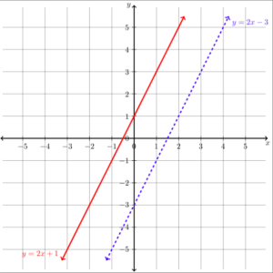
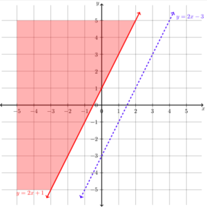
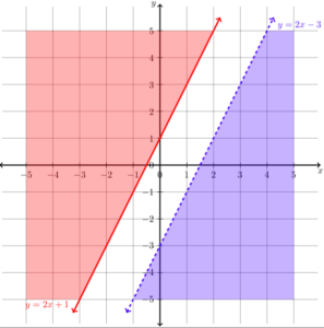
In the next example, we will show the solution to a system of two inequalities whose boundary lines are parallel to each other.  When the graphs of a system of two linear equations are parallel to each other, we found that there was no solution to the system.  We will get a similar result for the following system of linear inequalities.

Examples

Graph the system [latex]\begin{array}{c}y\ge2x+1\\y\lt2x-3\end{array}[/latex]

Show Solution

The boundary lines for this system are parallel to each other, note how they have the same slopes.

[latex]\begin{array}{c}y=2x+1\\y=2x-3\end{array}[/latex]

Plotting the boundary lines will give the graph below. Note that the inequality [latex]y\lt2x-3[/latex] requires that we draw a dashed line, while the inequality [latex]y\ge2x+1[/latex] will require a solid line.

Now we need to add the regions that represent the inequalities.  For the inequality [latex]y\ge2x+1[/latex] we can test a point on either side of the line to see which region to shade. Let’s test [latex]\left(0,0\right)[/latex] to make it easy.

Substitute [latex]\left(0,0\right)[/latex] into [latex]y\ge2x+1[/latex]

[latex]\begin{array}{c}y\ge2x+1\\0\ge2\left(0\right)+1\\0\ge{1}\end{array}[/latex]

This is not true, so we know that we need to shade the other side of the boundary line for the inequality  [latex]y\ge2x+1[/latex]. The graph will now look like this:

Now let’s shade the region that shows the solutions to the inequality [latex]y\lt2x-3[/latex].  Again, we can pick [latex]\left(0,0\right)[/latex] to test because it makes easy algebra.

Substitute [latex]\left(0,0\right)[/latex] into [latex]y\lt2x-3[/latex]

[latex]\begin{array}{c}y\lt2x-3\\0\lt2\left(0,\right)x-3\\0\lt{-3}\end{array}[/latex]

This is not true, so we know that we need to shade the other side of the boundary line for the inequality[latex]y\lt2x-3[/latex]. The graph will now look like this:

This system of inequalities shares no points in common.

In the following examples, we will continue to practice graphing the solution region for systems of linear inequalities.  We will also graph the solutions to a system that includes a compound inequality.

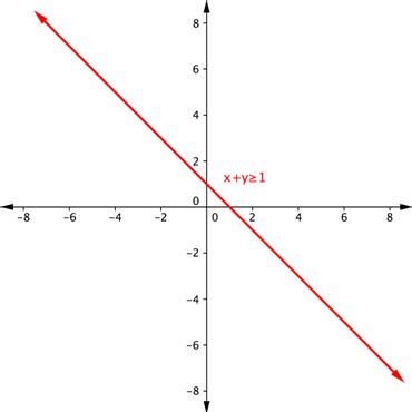
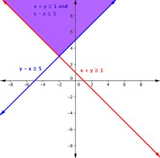
Example

Shade the region of the graph that represents solutions for both inequalities.  [latex]x+y\geq 1[/latex] and [latex]y -x\geq 5[/latex].

Show Solution

Graph one inequality. First graph the boundary line, using a table of values, intercepts, or any other method you prefer. The boundary line for [latex]x+y\geq1[/latex] is [latex]x+y=1[/latex], or [latex]y=−x+1[/latex]. Since the equal sign is included with the greater than sign, the boundary line is solid.

Find an ordered pair on either side of the boundary line. Insert the x– and y-values into the inequality [latex]x+y\geq1[/latex] and see which ordered pair results in a true statement.

[latex]\begin{array}{r}\text{Test }1:\left(−3,0\right)\\x+y\geq1\\−3+0\geq1\\−3\geq1\\\text{FALSE}\\\\\text{Test }2:\left(4,1\right)\\x+y\geq1\\4+1\geq1\\5\geq1\\\text{TRUE}\end{array}[/latex]

Since [latex](4, 1)[/latex] results in a true statement, the region that includes [latex](4, 1)[/latex] should be shaded.

Do the same with the second inequality. Graph the boundary line, then test points to find which region is the solution to the inequality. In this case, the boundary line is [latex]y–x=5\left(\text{or }y=x+5\right)[/latex] and is solid. Test point (−3, 0) is not a solution of [latex]y–x\geq5[/latex], and test point (0, 6) is a solution.

Answer

The purple region in this graph shows the set of all solutions of the system.

The videos that follow show more examples of graphing the solution set of a system of linear inequalities.

The system in our last example includes a compound inequality.  We will see that you can treat a compound inequality like two lines when you are graphing them.

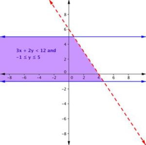
Example

Find the solution to the system [latex]3x + 2y < 12[/latex] and [latex]−1\leq y \leq 5[/latex].

Show Answer

Graph one inequality. First graph the boundary line, then test points.

Remember, because the inequality [latex]3x + 2y<12[/latex] does not include the equal sign, draw a dashed border line.

Testing a point like [latex](0, 0)[/latex] will show that the area below the line is the solution to this inequality.

The inequality [latex]−1\leq y \leq 5[/latex] is actually two inequalities: [latex]−1\leq y[/latex], and [latex]y \leq 5[/latex]. Another way to think of this is y must be between −1 and 5. The border lines for both are horizontal. The region between those two lines contains the solutions of [latex]−1\leq y\leq 5[/latex]. We make the lines solid because we also want to include [latex]y = −1[/latex] and [latex]y = 5[/latex].

Graph this region on the same axes as the other inequality.

The purple region in this graph shows the set of all solutions of the system.

Answer

In the video that follows, we show how to solve another system of inequalities.

(6.4.6) – Applications of systems of linear inequalities

In our first example we will show how to write and graph a system of linear inequalities that models the amount of sales needed to obtain a specific amount of money.

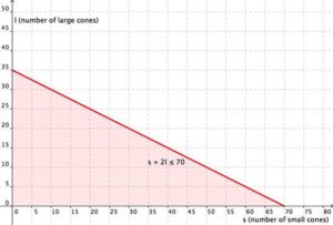
Example

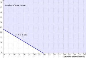
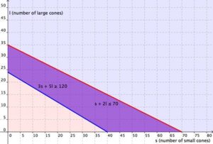
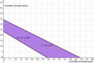
Cathy is selling ice cream cones at a school fundraiser. She is selling two sizes: small (which has 1 scoop) and large (which has 2 scoops). She knows that she can get a maximum of 70 scoops of ice cream out of her supply. She charges $3 for a small cone and $5 for a large cone.

Cathy wants to earn at least $120 to give back to the school. Write and graph a system of inequalities that models this situation.

Show Answer

First, identify the variables. There are two variables: the number of small cones and the number of large cones.

[latex]s[/latex] = small cone

[latex]l[/latex] = large cone

Write the first equation: the maximum number of scoops she can give out. The scoops she has available (70) must be greater than or equal to the number of scoops for the small cones [latex](s)[/latex] and the large cones [latex](2l)[/latex] she sells.

[latex]s+2l\le70[/latex]

Write the second equation: the amount of money she raises. She wants the total amount of money earned from small cones [latex](3s)[/latex] and large cones [latex](5l)[/latex] to be at least $120.

[latex]3s+5l\ge120[/latex]

Write the system.

[latex]\begin{cases}s+2l\le70\\3s+5l\ge120\end{cases}[/latex]

Now graph the system. The variables [latex]x[/latex] and [latex]y[/latex] have been replaced by [latex]s[/latex] and [latex]l[/latex]; graph s along the [latex]x[/latex]-axis, and [/latex]l[/latex] along the [/latex]y[/latex]-axis.

First graph the region [latex]s + 2l� \leq 70[/latex]. Graph the boundary line and then test individual points to see which region to shade. The graph is shown below.

Now graph the region [latex]3s+5l\ge120[/latex] Graph the boundary line and then test individual points to see which region to shade. The graph is shown below.

Graphing the regions together, you find the following:

And represented just as the overlapping region, you have:

Answer

The region in purple is the solution. As long as the combination of small cones and large cones that Cathy sells can be mapped in the purple region, she will have earned at least $120 and not used more than 70 scoops of ice cream.

In a previous example for finding a solution to a system of linear equations, we introduced a manufacturer’s cost and revenue equations:

Cost: [latex]y=0.85x+35,000[/latex]

Revenue: [latex]y=1.55x[/latex]

The cost equation is shown in blue in the graph below, and the revenue equation is graphed in orange.The point at which the two lines intersect is called the break-even point, we learned that this is the solution to the system of linear equations that in this case comprise the cost and revenue equations.

The shaded region to the right of the break-even point represents quantities for which the company makes a profit. The region to the left represents quantities for which the company suffers a loss.

In the next example, you will see how the information you learned about systems of linear inequalities can be applied to answering questions about cost and revenue.

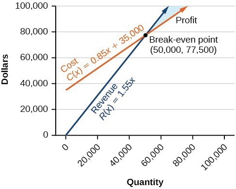
Note how the blue shaded region between the Cost and Revenue equations is labeled Profit. This is the “sweet spot” that the company wants to achieve where they produce enough bike frames at a minimal enough cost to make money. They don’t want more money going out than coming in!

Example

Define the profit region for the skateboard manufacturing business using inequalities, given the system of linear equations:

Cost: [latex]y=0.85x+35,000[/latex]

Revenue: [latex]y=1.55x[/latex]

Show Solution

We know that graphically,  solutions to linear inequalities are entire regions, and we learned how to graph systems of linear inequalities earlier in this module. Based on the graph below and the equations that define cost and revenue, we can use inequalities to define the region for which the skateboard manufacturer will make a profit.

Let’s start with the revenue equation.  We know that the break even point is at (50,000, 77,500) and the profit region is the blue area.  If we choose a point in the region and test it like we did for finding solution regions to inequalities, we will know which kind of inequality sign to use.

Let’s test the point [latex]\left(65,00,100,000\right)[/latex] in both equations to determine which inequality sign to use.

Cost:

[latex]\begin{array}{l}y=0.85x+{35,000}\\{100,000}\text{ ? }0.85\left(65,000\right)+35,000\\100,000\text{ ? }90,250\end{array}[/latex]

We need to use > because 100,000 is greater than 90,250

The cost inequality that will ensure the company makes profit – not just break even – is [latex]y>0.85x+35,000[/latex]

Now test the point in the revenue equation:

Revenue:

[latex]\begin{array}{l}y=1.55x\\100,000\text{ ? }1.55\left(65,000\right)\\100,000\text{ ? }100,750\end{array}[/latex]

We need to use < because 100,000 is less than 100,750

The revenue inequality that will ensure the company makes profit – not just break even – is [latex]y<1.55x[/latex]

The systems of inequalities that defines the profit region for the bike manufacturer:

[latex]\begin{array}{l}y>0.85x+35,000\\y<1.55x\end{array}[/latex]

Answer

The cost to produce 50,000 units is $77,500, and the revenue from the sales of 50,000 units is also $77,500. To make a profit, the business must produce and sell more than 50,000 units. The system of linear inequalities that represents the number of units that the company must produce in order to earn a profit is:

[latex]\begin{array}{l}y>0.85x+35,000\\y<1.55x\end{array}[/latex]

In the following video you will see an example of how to find the break even point for a small sno-cone business.

And here is one more video example of solving an application using a sustem of linear inequalities.

We have seen that systems of linear equations and inequalities can help to define market behaviors that are very helpful to businesses.  The intersection of cost and revenue equations gives the break even point, and also helps define the region for which a company will make a profit.