(3.2.1) – Graphing functions using a table of values

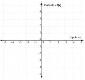
When both the input (independent variable) and the output (dependent variable) are real numbers, a function can be represented by a coordinate graph. The input is plotted on the horizontal x-axis and the output is plotted on the vertical y-axis.

A helpful first step in graphing a function is to make a table of values. This is particularly useful when you don’t know the general shape the function will have. You probably already know that a linear function will be a straight line, but let’s make a table first to see how it can be helpful.

When making a table, it’s a good idea to include negative values, positive values, and zero to ensure that you do have a linear function.

Graphing linear functions

Make a table of values for [latex]f(x)=3x+2[/latex].

Make a two-column table. Label the columns x and f(x).

Choose several values for x and put them as separate rows in the x column. These are YOUR CHOICE – there is no “right” or “wrong” values to pick, just go for it.

Tip: It’s always good to include 0, positive values, and negative values, if you can.

Evaluate the function for each value of x, and write the result in the f(x) column next to the x value you used.

When [latex]x=0[/latex], [latex]f(0)=3(0)+2=2[/latex],

[latex]f(1)=3(1)+2=5[/latex],

[latex]f(−1)=3(−1)+2=−3+2=−1[/latex], and so on.

(Note that your table of values may be different from someone else’s. You may each choose different numbers for x.)

Now that you have a table of values, you can use them to help you draw both the shape and location of the function. Important: The graph of the function will show all possible values of x and the corresponding values of y. This is why the graph is a line and not just the dots that make up the points in our table.

Graph [latex]f(x)=3x+2[/latex].
Using the table of values we created above you can think of f(x) as y, each row forms an ordered pair that you can plot on a coordinate grid.

Plot the points.

Since the points lie on a line, use a straight edge to draw the line. Try to go through each point without moving the straight edge.

Let’s try another one. Before you look at the answer, try to make the table yourself and draw the graph on a piece of paper.

Example

Graph [latex]f(x)=−x+1[/latex].

Show Solution

Start with a table of values. You can choose different values for x, but once again, it’s helpful to include 0, some positive values, and some negative values.

If you think of f(x) as y, each row forms an ordered pair that you can plot on a coordinate grid.

[latex]f(−2)=−(−2)+1=2+1=3\\f(−1)=−(−1)+1=1+1=2\\f(0)=−(0)+1=0+1=1\\f(1)=−(1)+1=−1+1=0\\f(2)=−(2)+1=−2+1=−1[/latex]

x	f(x)
[latex]−2[/latex]	[latex]3[/latex]
[latex]−1[/latex]	[latex]2[/latex]
[latex]0[/latex]	[latex]1[/latex]
[latex]1[/latex]	[latex]0[/latex]
[latex]2[/latex]	[latex]−1[/latex]

Plot the points.

Answer

Since the points lie on a line, use a straight edge to draw the line. Try to go through each point without moving the straight edge.

In the following video we show another example of how to graph a linear function on a set of coordinate axes.

These graphs are representations of a linear function. Remember that a function is a correspondence between two variables, such as x and y. These will be discussed in further detail in the next module.

Graphing quadratic functions

Quadratic functions can also be graphed. It’s helpful to have an idea what the shape should be, so you can be sure that you’ve chosen enough points to plot as a guide. Let’s start with the most basic quadratic function, [latex]f(x)=x^{2}[/latex].
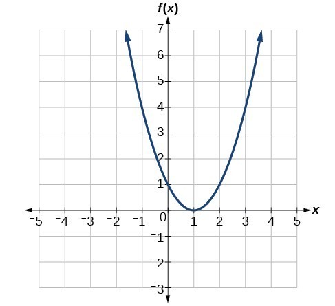
Graph [latex]f(x)=x^{2}[/latex].
Start with a table of values. Then think of the table as ordered pairs.

Plot the points [latex](-2,4), (-1,1), (0,0), (1,1), (2,4)[/latex]

Since the points are not on a line, you can’t use a straight edge. Connect the points as best you can, using a smooth curve (not a series of straight lines). You may want to find and plot additional points (such as the ones in blue here). Placing arrows on the tips of the lines implies that they continue in that direction forever.

Notice that the shape is like the letter U. This is called a parabola. One-half of the parabola is a mirror image of the other half. The line that goes down the middle is called the line of reflection, in this case that line is they y-axis. The lowest point on this graph is called the vertex.

In the following video we show an example of plotting a quadratic function using a table of values.

The equations for quadratic functions have the form [latex]f(x)=ax^{2}+bx+c[/latex] where [latex] a\ne 0[/latex]. In the basic graph above, [latex]a=1[/latex], [latex]b=0[/latex], and [latex]c=0[/latex].

Changing a changes the width of the parabola and whether it opens up ([latex]a>0[/latex]) or down ([latex]a<0[/latex]). If a is positive, the vertex is the lowest point, if a is negative, the vertex is the highest point. In the following example, we show how changing the value of a will affect the graph of the function.

Example

Match the following functions with their graph.

a) [latex] \displaystyle f(x)=3{{x}^{2}}[/latex]

b) [latex] \displaystyle f(x)=-3{{x}^{2}}[/latex]

c)[latex] \displaystyle f(x)=\frac{1}{2}{{x}^{2}}[/latex]

a)

b)

c)

Show Answer

Function a) [latex] \displaystyle f(x)=3{{x}^{2}}[/latex] means that inputs are squared and then multiplied by three, so the outputs will be greater than they would have been for [latex]f(x)=x^2[/latex].  This results in a parabola that has been squeezed, so the graph b) is the best match for this function.

Function b) [latex] \displaystyle f(x)=-3{{x}^{2}}[/latex] means that inputs are squared and then multiplied by negative three, so the outputs will be greater than they would have been for [latex]f(x)=x^2[/latex] so graph a)  is the best match for this function.

Function c) [latex] \displaystyle f(x)=\frac{1}{2}{{x}^{2}}[/latex] means that inputs are squared then multiplied by [latex]\frac{1}{2}[/latex], so the outputs are less than they would be for [latex]f(x)=x^2[/latex].  This results in a parabola that has been opened wider than[latex]f(x)=x^2[/latex]. Graph c) is the best match for this function.

Answer

Function a) matches graph b)

Function b) matches graph a)

Function c) matches graph c)

If there is no b term, changing c moves the parabola up or down so that the y intercept is (0, c). In the next example we show how changes to c affect the graph of the function.

Example

Match the following functions with their graph.

a) [latex] \displaystyle f(x)={{x}^{2}}+3[/latex]

b) [latex] \displaystyle f(x)={{x}^{2}}-3[/latex]

a)

b)

Show Answer

Function a) [latex] \displaystyle f(x)={{x}^{2}}+3[/latex] means square the inputs then add three, so every output will be moved up 3 units. the graph that matches this function best is b)

Function b) [latex] \displaystyle f(x)={{x}^{2}}-3[/latex]  means square the inputs then subtract three, so every output will be moved down 3 units. the graph that matches this function best is a)

(3.2.2) – Finding Function Values from a Graph

Evaluating a function using a graph also requires finding the corresponding output value for a given input value, only in this case, we find the output value by looking at the graph. Solving a function equation using a graph requires finding all instances of the given output value on the graph and observing the corresponding input value(s).

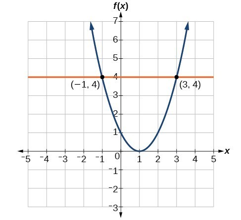
Example: Reading Function Values from a Graph

Given the graph below,

1. Evaluate [latex]f\left(2\right)[/latex].
2. Solve [latex]f\left(x\right)=4[/latex].

Solution

1. To evaluate [latex]f\left(2\right)[/latex], locate the point on the curve where [latex]x=2[/latex], then read the y-coordinate of that point. The point has coordinates [latex]\left(2,1\right)[/latex], so [latex]f\left(2\right)=1[/latex].
2. To solve [latex]f\left(x\right)=4[/latex], we find the output value [latex]4[/latex] on the vertical axis. Moving horizontally along the line [latex]y=4[/latex], we locate two points of the curve with output value [latex]4:[/latex] [latex]\left(-1,4\right)[/latex] and [latex]\left(3,4\right)[/latex]. These points represent the two solutions to [latex]f\left(x\right)=4:[/latex] [latex]x=-1[/latex] or [latex]x=3[/latex]. This means [latex]f\left(-1\right)=4[/latex] and [latex]f\left(3\right)=4[/latex], or when the input is [latex]-1[/latex] or [latex]\text{3,}[/latex] the output is [latex]\text{4}\text{.}[/latex]See Figure 8.

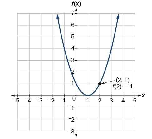
Try It

Using the graph, solve [latex]f\left(x\right)=1[/latex].

Solution

[latex]x=0[/latex] or [latex]x=2[/latex]

(3.2.3) – Vertical line test

When both the independent quantity (input) and the dependent quantity (output) are real numbers, a function can be represented by a graph in the coordinate plane. The independent value is plotted on the x-axis and the dependent value is plotted on the y-axis. The fact that each input value has exactly one output value means graphs of functions have certain characteristics. For each input on the graph, there will be exactly one output. For a function defined as [latex]y = f(x)[/latex], or [latex]y[/latex] is a function of [latex]x[/latex], we would write ordered pairs [latex](x, f(x))[/latex] using function notation instead of [latex](x,y)[/latex] as you may have seen previously.

We can identify whether the graph of a relation represents a function because for each x-coordinate there will be exactly one y-coordinate.

When a vertical line is placed across the plot of this relation, it does not intersect the graph more than once for any values of [latex]x[/latex].

If, on the other hand, a graph shows two or more intersections with a vertical line, then an input (x-coordinate) can have more than one output (y-coordinate), and [latex]y[/latex] is not a function of [latex]x[/latex]. Examining the graph of a relation to determine if a vertical line would intersect with more than one point is a quick way to determine if the relation shown by the graph is a function. This method is often called the “vertical line test.”

You try it.

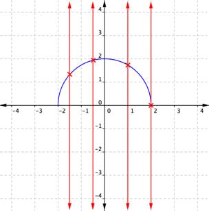
Example

Use the vertical line test to determine whether the relation plotted on this graph is a function.

Show Answer

This relationship cannot be a function, because some of the x-coordinates have two corresponding y-coordinates.

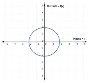
The vertical line method can also be applied to a set of ordered pairs plotted on a coordinate plane to determine if the relation is a function.

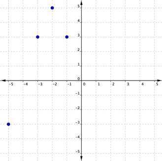
Example

Consider the ordered pairs

[latex]\{(−1,3),(−2,5),(−3,3),(−5,−3)\}[/latex], plotted on the graph below. Use the vertical line test to determine whether the set of ordered pairs represents a function.

Show Answer

Drawing vertical lines through each point results in each line only touching one point. This means that none of the x-coordinates have two corresponding y-coordinates, so this is a function.

In another set of ordered pairs, [latex]\{(3,−1),(5,−2),(3,−3),(−3,5)\}[/latex], one of the inputs, 3, can produce two different outputs, [latex]−1[/latex] and [latex]−3[/latex]. You know what that means—this set of ordered pairs is not a function. A plot confirms this.

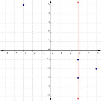
Notice that a vertical line passes through two plotted points. One x-coordinate has multiple y-coordinates. This relation is not a function.

In the following video we show another example of determining whether a graph represents a function using the vertical line test.