Learning Objectives
- (4.1.1) – Define slope for a linear function
- (4.1.2) – Calculate slope given two points
- (4.1.3) – Graph a linear function using the standard form
- (4.1.4) – Graph a linear function using the slope and y-intercept

Imagine placing a plant in the ground one day and finding that it has doubled its height just a few days later. Although it may seem incredible, this can happen with certain types of bamboo species. These members of the grass family are the fastest-growing plants in the world. One species of bamboo has been observed to grow nearly 1.5 inches every hour. In a twenty-four hour period, this bamboo plant grows about 36 inches, or an incredible 3 feet! A constant rate of change, such as the growth cycle of this bamboo species, is a linear function.
One well known form for writing linear functions is known as the slope-intercept form, where [latex]x[/latex] is the input value, [latex]m[/latex] is the rate of change, and [latex]b[/latex] is the initial value of the dependant variable.
[latex]\begin{array}{cc}\text{Equation form}\hfill & y=mx+b\hfill \\ \text{Function notation}\hfill & f\left(x\right)=mx+b\hfill \end{array}[/latex]
(4.1.1) – Define slope for a linear function
We often need to calculate the slope given input and output values. Given two values for the input, [latex]{x}_{1}[/latex] and [latex]{x}_{2}[/latex], and two corresponding values for the output, [latex]{y}_{1}[/latex] and [latex]{y}_{2}[/latex] —which can be represented by a set of points, [latex]\left({x}_{1}\text{, }{y}_{1}\right)[/latex] and [latex]\left({x}_{2}\text{, }{y}_{2}\right)[/latex]—we can calculate the slope [latex]m[/latex], as follows
[latex]\displaystyle m=\frac{\text{change in output (rise)}}{\text{change in input (run)}}=\frac{\Delta y}{\Delta x}=\frac{{y}_{2}-{y}_{1}}{{x}_{2}-{x}_{1}}[/latex]
where [latex]\Delta y[/latex] is the vertical displacement and [latex]\Delta x[/latex] is the horizontal displacement. Note in function notation two corresponding values for the output [latex]{y}_{1}[/latex] and [latex]{y}_{2}[/latex] for the function [latex]f[/latex], [latex]{y}_{1}=f\left({x}_{1}\right)[/latex] and [latex]{y}_{2}=f\left({x}_{2}\right)[/latex], so we could equivalently write
[latex]\displaystyle m=\frac{f\left({x}_{2}\right)-f\left({x}_{1}\right)}{{x}_{2}-{x}_{1}}[/latex]
The graph in Figure 5 indicates how the slope of the line between the points, [latex]\left({x}_{1,}{y}_{1}\right)[/latex] and [latex]\left({x}_{2,}{y}_{2}\right)[/latex], is calculated. Recall that the slope measures steepness. The greater the absolute value of the slope, the steeper the line is.
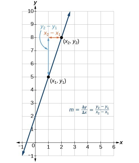
The slope of a function is calculated by the change in [latex]y[/latex] divided by the change in [latex]x[/latex]. It does not matter which coordinate is used as the [latex]\left({x}_{2,\text{ }}{y}_{2}\right)[/latex] and which is the [latex]\left({x}_{1},\text{ }{y}_{1}\right)[/latex], as long as each calculation is started with the elements from the same coordinate pair.
The units for slope are always [latex]\frac{\text{units for the output}}{\text{units for the input}}[/latex] Think of the units as the change of output value for each unit of change in input value. An example of slope could be miles per hour or dollars per day. Notice the units appear as a ratio of units for the output per units for the input.
(4.1.2) – Calculate Slope Given Two Points
Calculate Slope
The slope, or rate of change, of a function [latex]m[/latex] can be calculated according to the following:
[latex]\displaystyle m=\frac{\text{change in output (rise)}}{\text{change in input (run)}}=\frac{\Delta y}{\Delta x}=\frac{{y}_{2}-{y}_{1}}{{x}_{2}-{x}_{1}}[/latex]
where [latex]{x}_{1}[/latex] and [latex]{x}_{2}[/latex] are input values, [latex]{y}_{1}[/latex] and [latex]{y}_{2}[/latex] are output values.
When the slope of a linear function is positive, the line is moving in an uphill direction across the coordinate axes. This is also called an increasing linear function. Likewise, a decreasing linear function is one whose slope is negative. The graph of a decreasing linear function is a line moving in a downhill direction across the coordinate axes.
In mathematical terms,
For a linear function [latex]f(x)=mx+b[/latex] if [latex]m>0[/latex], then [latex]f(x)[/latex] is an increasing function.
For a linear function [latex]f(x)=mx+b[/latex] if [latex]m<0[/latex], then [latex]f(x)[/latex] is a decreasing function. For a linear function [latex]f(x)=mx+b[/latex] if [latex]m=0[/latex], then [latex]f(x)[/latex] is a constant function. Sometimes we say this is neither increasing nor decreasing. In the following example we will first find the slope of a linear function through two points, then determine whether the line is increasing, decreasing, or neither.
Example
If [latex]f\left(x\right)[/latex] is a linear function, and [latex]\left(3,-2\right)[/latex] and [latex]\left(8,1\right)[/latex] are points on the line, find the slope. Is this function increasing or decreasing?
In the following video we show examples of how to find the slope of a line passing between two points, then determine whether the line is increasing, decreasing or neither.
Example
The population of a city increased from 23,400 to 27,800 between 2008 and 2012. Find the change of population per year if we assume the change was constant from 2008 to 2012.
In the next video we show an example where we determine the increase in cost for producing solar panels given two data points.
The following video provides na example of how to write a function that will give the cost in dollars for a given number of credit hours taken, x.
(4.1.3) – Graph Linear Functions Using the Standard Form
Standard Form of a Line
Another way that we can represent the equation of a line is in standard form. Standard form is given as
[latex]Ax+By=C[/latex]
where [latex]A[/latex], [latex]B[/latex], and [latex]C[/latex] are integers. The x- and y-terms are on one side of the equal sign and the constant term is on the other side.
Using intercepts to graph a line in standard form
The intercepts of a line are the points where the line intercepts, or crosses, the horizontal and vertical axes. To help you remember what “intercept” means, think about the word “intersect.” The two words sound alike and in this case mean the same thing.
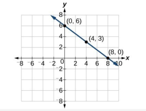
The straight line on the graph below intercepts the two coordinate axes. The point where the line crosses the x-axis is called the x-intercept. The y-intercept is the point where the line crosses the y-axis.
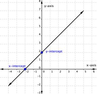
The x-intercept above is the point [latex](−2,0)[/latex]. The y-intercept above is the point (0, 2).
Notice that the y-intercept always occurs where [latex]x=0[/latex], and the x-intercept always occurs where [latex]y=0[/latex].
To find the x– and y-intercepts of a linear equation, you can substitute 0 for y and for x respectively.
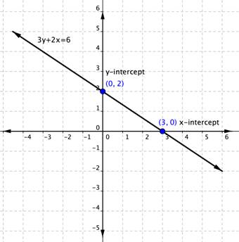
For example, the linear equation [latex]3y+2x=6[/latex] has an x intercept when [latex]y=0[/latex], so [latex]3\left(0\right)+2x=6\\[/latex].
[latex]\begin{array}{r}2x=6\\x=3\end{array}[/latex]
The x-intercept is [latex](3,0)[/latex].
Likewise the y-intercept occurs when [latex]x=0[/latex].
[latex]\begin{array}{r}3y+2\left(0\right)=6\\3y=6\\y=2\end{array}[/latex]
The y-intercept is [latex](0,2)[/latex].
You can use intercepts to graph linear equations. Once you have found the two intercepts, draw a line through them.
Let’s do it with the equation [latex]3y+2x=6[/latex]. You figured out that the intercepts of the line this equation represents are [latex](0,2)[/latex] and [latex](3,0)[/latex]. That’s all you need to know.
Example
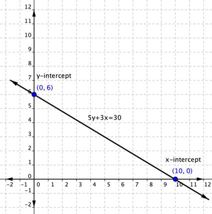
Graph [latex]5y+3x=30[/latex] using the x and y-intercepts.
(4.1.4) – Graph Linear Functions Using Slope and y-Intercept
Another way to graph a linear function is by using its slope m, and y-intercept.
Let’s consider the following function.
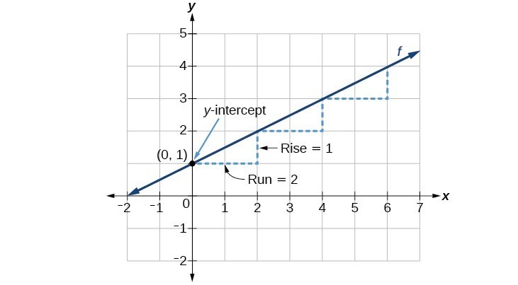
[latex]\displaystyle f\left(x\right)=\frac{1}{2}x+1[/latex]
The slope is [latex]\frac{1}{2}[/latex]. Because the slope is positive, we know the graph will slant upward from left to right. The y-intercept is the point on the graph when x = 0. The graph crosses the y-axis at (0, 1). Now we know the slope and the y-intercept. We can begin graphing by plotting the point (0, 1) We know that the slope is rise over run, [latex]m=\frac{\text{rise}}{\text{run}}[/latex]. From our example, we have [latex]m=\frac{1}{2}[/latex], which means that the rise is 1 and the run is 2. So starting from our y-intercept (0, 1), we can rise 1 and then run 2, or run 2 and then rise 1. We repeat until we have a few points, and then we draw a line through the points as shown in the graph below.
A General Note: Graphical Interpretation of a Linear Function
In the equation [latex]f\left(x\right)=mx+b[/latex]
- b is the y-intercept of the graph and indicates the point (0, b) at which the graph crosses the y-axis.
- m is the slope of the line and indicates the vertical displacement (rise) and horizontal displacement (run) between each successive pair of points. Recall the formula for the slope:
[latex]\displaystyle m=\frac{\text{change in output (rise)}}{\text{change in input (run)}}=\frac{\Delta y}{\Delta x}=\frac{{y}_{2}-{y}_{1}}{{x}_{2}-{x}_{1}}[/latex]
All linear functions cross the y-axis and therefore have y-intercepts. (Note: A vertical line parallel to the y-axis does not have a y-intercept, but it is not a function.)
How To: Given the equation for a linear function, graph the function using the y-intercept and slope.
- Evaluate the function at an input value of zero to find the y-intercept.
- Identify the slope as the rate of change of the input value.
- Plot the point represented by the y-intercept.
- Use [latex]\frac{\text{rise}}{\text{run}}[/latex] to determine at least two more points on the line.
- Sketch the line that passes through the points.
Example
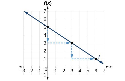
Graph [latex]\displaystyle f\left(x\right)=-\frac{2}{3}x+5[/latex] using the y-intercept and slope.
In the following video we show another example of how to graph a linear function given the y-intercepts and the slope.
In the last example we will show how to graph another linear function using the slope and y-intercept.
Example
Graph [latex]\displaystyle f\left(x\right)=-\frac{3}{4}x+6[/latex] using the slope and y-intercept.
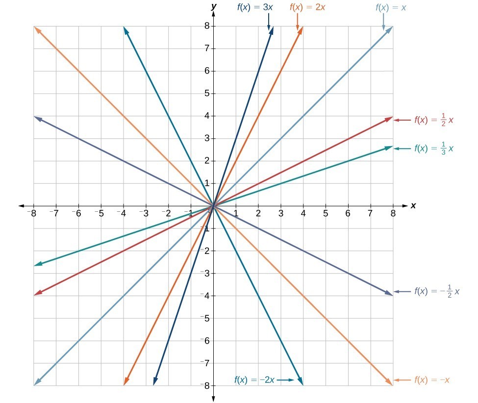
Example
The following figure illustrates the graphs of lines going through the origin [latex](0,0)[/latex]. Notice, the larger the absolute value of m, the steeper the slope.
Candela Citations
- Revision and Adaptation. Provided by: Lumen Learning. License: CC BY: Attribution
- Write and Graph a Linear Function by Making a Table of Values (Intro). Authored by: James Sousa (Mathispower4u.com) for Lumen Learning. Located at: https://youtu.be/X3Sx2TxH-J0. License: CC BY: Attribution
- Graph a Linear Function as a Transformation of f(x)=x. Authored by: James Sousa (Mathispower4u.com) for Lumen Learning. Located at: https://youtu.be/h9zn_ODlgbM. License: CC BY: Attribution
- Interactive Linear Graphing. Authored by: Tatyana Khodorovskiy. Provided by: (with Desmos Graphing). Located at: https://www.desmos.com/calculator/r8ddrnhgwv. License: Public Domain: No Known Copyright
- Precalculus. Authored by: Jay Abramson, et al.. Provided by: OpenStax. Located at: http://cnx.org/contents/fd53eae1-fa23-47c7-bb1b-972349835c3c@5.175. License: CC BY: Attribution
- Ex: Find the Slope Given Two Points and Describe the Line. Authored by: James Sousa (Mathispower4u.com) for Lumen Learning. Located at: https://youtu.be/in3NTcx11I8. License: CC BY: Attribution
- Ex: Slope Application Involving Production Costs. Authored by: James Sousa (Mathispower4u.com) for Lumen Learning. Located at: https://youtu.be/4RbniDgEGE4. License: CC BY: Attribution
- Ex: Graph a Line and ID the Slope and Intercepts (Fraction Slope). Authored by: James Sousa (Mathispower4u.com) for Lumen Learning. Located at: https://youtu.be/N6lEPh11gk8. License: CC BY: Attribution
- Graph Linear Equations Using Intercepts. Authored by: James Sousa (Mathispower4u.com) . Located at: https://youtu.be/k8r-q_T6UFk. License: CC BY: Attribution