earning Objectives
- (7.2.1) – Identify polynomial functions
- (7.2.2) – Identify the degree and leading coefficient of a polynomial function
- (7.2.3) – Identify graphs of even and odd polynomial functions
- (7.2.4) – Use the leading coefficient test to determine the end behavior of polynomials
(7.2.1) – Identify polynomial functions
We have introduced polynomials and functions, so now we will combine these ideas to describe polynomial functions. Polynomials are algebraic expressions that are created by summing monomial terms, such as [latex]-3x^2[/latex], where the exponents are only integers. Functions are a specific type of relation in which each input value has one and only one output value. Polynomial functions have all of these characteristics as well as a domain and range, and corresponding graphs. In this section we will identify and evaluate polynomial functions. Because of the form of a polynomial function, we can see an infinite variety in the number of terms and the power of the variable.
When we introduced polynomials, we presented the following: [latex]4x^3-9x^2 6x[/latex]. We can turn this into a polynomial function by using function notation:
[latex]f(x)=4x^3-9x^2 6x[/latex]
Polynomial functions are written with the leading term first, and all other terms in descending order as a matter of convention. In the first example, we will identify some basic characteristics of polynomial functions.
Example
Which of the following are polynomial functions?
In the following video you will see additional examples of how to identify a polynomial function using the definition.
(7.2.2) – Identify the degree and leading coefficient of a polynomial function
Just as we identified the degree of a polynomial, we can identify the degree of a polynomial function. To review: the degree of the polynomial is the highest power of the variable that occurs in the polynomial; the leading term is the term containing the highest power of the variable, or the term with the highest degree. The leading coefficient is the coefficient of the leading term.
Example
Identify the degree, leading term, and leading coefficient of the following polynomial functions.
In the next video we will show more examples of how to identify the degree, leading term and leading coefficient of a polynomial function.
(7.2.3) – Identify graphs of even and odd polynomial functions
Plotting polynomial functions using tables of values can be misleading because of some of the inherent characteristics of polynomials. Additionally, the algebra of finding points like x-intercepts for higher degree polynomials can get very messy and oftentimes impossible to find by hand. We have therefore developed some techniques for describing the general behavior of polynomial graphs.
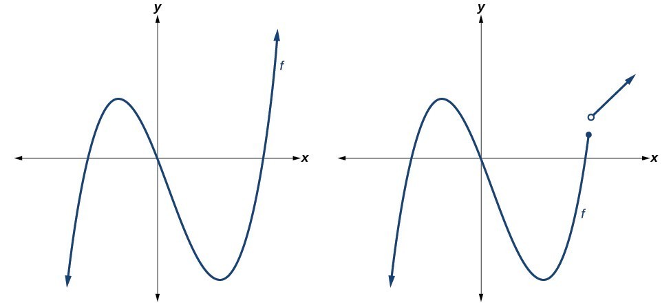
Polynomial functions of degree 2 or more have graphs that do not have sharp corners these types of graphs are called smooth curves. Polynomial functions also display graphs that have no breaks. Curves with no breaks are called continuous. The figure below shows a graph that represents a polynomial function and a graph that represents a function that is not a polynomial.
Now you try it.
Example
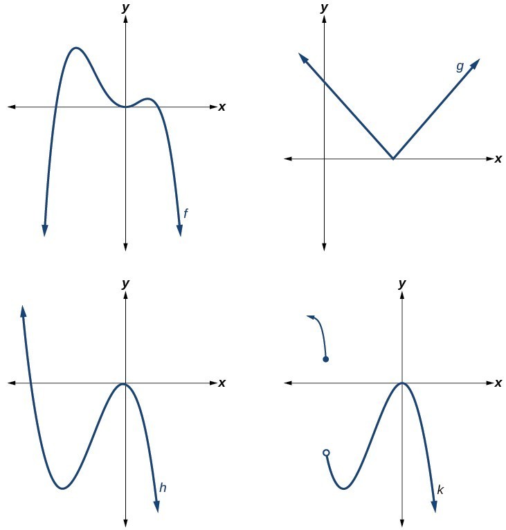
Which of the graphs below represents a polynomial function?
Q & A
Do all polynomial functions have as their domain all real numbers?
Yes. Any real number is a valid input for a polynomial function.
Identifying the shape of the graph of a polynomial function
Knowing the degree of a polynomial function is useful in helping us predict what it’s graph will look like. Because the power of the leading term is the highest, that term will grow significantly faster than the other terms as x gets very large or very small, so its behavior will dominate the graph. For any polynomial, the graph of the polynomial will match the end behavior of the term of highest degree.
As an example we compare the outputs of a degree 2 polynomial and a degree 5 polynomial in the following table.
| x | [latex]f(x)=2x^2-2x 4[/latex] | [latex]g(x)=x^5 2x^3-12x 3[/latex] |
| 1 | 4 | 8 |
| 10 | 184 | 98117 |
| 100 | 19804 | 9998001197 |
| 1000 | 1998004 | 9999980000000000 |
As the inputs for both functions get larger, the degree 5 polynomial outputs get much larger than the degree 2 polynomial outputs. This is why we use the leading term to get a rough idea of the behavior of polynomial graphs.
There are two other important features of polynomials that influence the shape of it’s graph. The first is whether the degree is even or odd, and the second is whether the leading term is negative.
Even degree polynomials
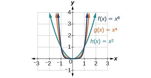
In the figure below, we show the graphs of [latex]f\left(x\right)={x}^{2},g\left(x\right)={x}^{4}[/latex] and [latex]\text{and}h\left(x\right)={x}^{6}[/latex], which are all have even degrees. Notice that these graphs have similar shapes, very much like that of a quadratic function. However, as the power increases, the graphs flatten somewhat near the origin and become steeper away from the origin.
Odd degree polynomials
The next figure shows the graphs of [latex]f\left(x\right)={x}^{3},g\left(x\right)={x}^{5},\text{and}h\left(x\right)={x}^{7}[/latex], which are all odd degree functions. 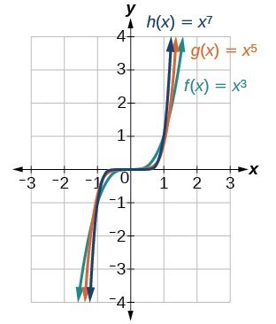
Notice that one arm of the graph points down and the other points up. This is because when your input is negative, you will get a negative output if the degree is odd. The following table of values shows this.
| x | [latex]f(x)=x^4[/latex] | [latex]h(x)=x^5[/latex] |
| -1 | 1 | -1 |
| -2 | 16 | -32 |
| -3 | 81 | -243 |
Now you try it.
Example
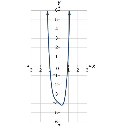
Identify whether graph represents a polynomial function that has a degree that is even or odd.
a)
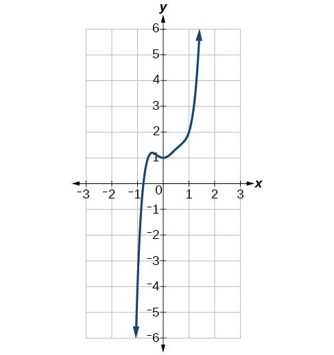
b)
The sign of the leading term
What would happen if we change the sign of the leading term of an even degree polynomial? For example, let’s say that the leading term of a polynomial is [latex]-3x^4[/latex]. We will use a table of values to compare the outputs for a polynomial with leading term [latex]-3x^4[/latex], and [latex]3x^4[/latex].
| x | [latex]-3x^4[/latex] | [latex]3x^4[/latex] |
| -2 | -48 | 48 |
| -1 | -3 | 3 |
| 0 | 0 | 0 |
| 1 | -3 | 3 |
| 2 | -48 | 48 |
Plotting these points on a grid leads to this plot, the red points indicate a negative leading coefficient, and the blue points indicate a positive leading coefficient:
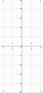
The negative sign creates a reflection of [latex]3x^4[/latex] across the [latex]x[/latex]-axis. The arms of a polynomial with a leading term of [latex]-3x^4[/latex] will point down, whereas the arms of a polynomial with leading term [latex]3x^4[/latex] will point up.
Now you try it.
Example
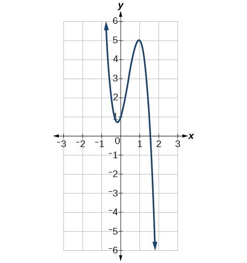
Identify whether the leading term is positive or negative and whether the degree is even or odd for the following graphs of polynomial functions.
a)
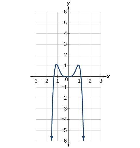
b)
(7.2.4) – Use the leading coefficient test to determine the end behavior of polynomials
As we have already learned, the behavior of a graph of a polynomial function of the form
[latex]f\left(x\right)={a}_{n}{x}^{n} {a}_{n - 1}{x}^{n - 1} ... {a}_{1}x {a}_{0}[/latex]
will either ultimately rise or fall as [latex]x[/latex] increases without bound and will either rise or fall as [latex]x[/latex] decreases without bound. This is because for very large inputs, say 100 or 1,000, the leading term dominates the size of the output. The same is true for very small inputs, say –100 or –1,000.
We call this behavior the end behavior of a function. When the leading term of a polynomial function, [latex]{a}_{n}{x}^{n}[/latex], is an even power function, as [latex]x[/latex] increases or decreases without bound, [latex]f\left(x\right)[/latex] increases without bound. When the leading term is an odd power function, as [latex]x[/latex] decreases without bound, [latex]f\left(x\right)[/latex] also decreases without bound; as [latex]x[/latex] increases without bound, [latex]f\left(x\right)[/latex] also increases without bound. If the leading term is negative, it will change the direction of the end behavior. Determining the end behavior from the sign of the leading coefficient and the degree of the leading term is called the leading coefficient test. The table below summarizes all four cases.
| Even Degree | Odd Degree |
|---|---|
 |
 |
| RISES LEFT, RISES RIGHT | FALLS LEFT, RISES RIGHT |
 |
 |
| FALLS LEFT, FALLS RIGHT | RISES LEFT, FALLS RIGHT |
Candela Citations
- Determine if a Function is a Polynomial Function. Authored by: James Sousa (Mathispower4u.com) for Lumen Learning. Located at: https://youtu.be/w02qTLrJYiQ. License: CC BY: Attribution
- Degree, Leading Term, and Leading Coefficient of a Polynomial Function. Authored by: James Sousa (Mathispower4u.com) for Lumen Learning. Located at: https://youtu.be/F_G_w82s0QA. License: CC BY: Attribution
- Revision and Adaptation. Provided by: Lumen Learning. License: CC BY: Attribution
- College Algebra. Authored by: Abramson, Jay, et al. Provided by: Open Stax. Located at: http://cnx.org/contents/9b08c294-057f-4201-9f48-5d6ad992740d@3.278:1/Preface. License: CC BY: Attribution. License Terms: Download fro free at : http://cnx.org/contents/9b08c294-057f-4201-9f48-5d6ad992740d@3.278:1/Preface