Learning Objectives
- (5.2.1) – Solve cost and revenue problems
- Specify what the variables in a cost/ revenue system of linear equations represent
- Determine and apply an appropriate method for solving the system
- (5.2.2) – Solve value problems with a system of linear equations
- (5.2.3) – Solve mixture problems with a system of linear equations
- (5.2.4) – Solve uniform motion problems with a system of linear equations
A skateboard manufacturer introduces a new line of boards. The manufacturer tracks its costs, which is the amount it spends to produce the boards, and its revenue, which is the amount it earns through sales of its boards. How can the company determine if it is making a profit with its new line? How many skateboards must be produced and sold before a profit is possible?
(credit: Thomas Sørenes)
(5.2.1) – Solve cost and revenue problems
Using what we have learned about systems of equations, we can return to the skateboard manufacturing problem at the beginning of the section. The skateboard manufacturer’s revenue function is the function used to calculate the amount of money that comes into the business. It can be represented by the equation [latex]R=xp[/latex], where [latex]x=[/latex] quantity and [latex]p=[/latex] price. The revenue function is shown in orange in the graph below.
The cost function is the function used to calculate the costs of doing business. It includes fixed costs, such as rent and salaries, and variable costs, such as utilities. The cost function is shown in blue in the graph below. The [latex]x[/latex] -axis represents quantity in hundreds of units. The y-axis represents either cost or revenue in hundreds of dollars.
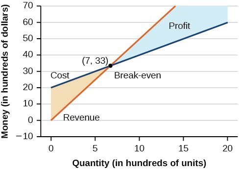
The point at which the two lines intersect is called the break-even point. We can see from the graph that if 700 units are produced, the cost is $3,300 and the revenue is also $3,300. In other words, the company breaks even if they produce and sell 700 units. They neither make money nor lose money.
The shaded region to the right of the break-even point represents quantities for which the company makes a profit. The shaded region to the left represents quantities for which the company suffers a loss. The profit function is the revenue function minus the cost function, written as [latex]P\left(x\right)=R\left(x\right)-C\left(x\right)[/latex]. Clearly, knowing the quantity for which the cost equals the revenue is of great importance to businesses.
Example
A business wants to manufacture bike frames. Before they start production, they need to make sure they can make a profit with the materials and labor force they have. Their accountant has given them a cost equation of [latex]y=0.85x+35,000[/latex] and a revenue equation of [latex]y=1.55x[/latex]:
- Interpret x and y for the cost equation
- Interpret x and y for the revenue equation
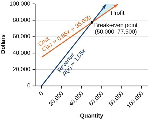
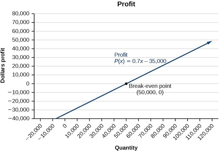
Example: Finding the Break-Even Point and the Profit Function Using Substitution
Given the cost function [latex]C\left(x\right)=0.85x+35,000[/latex] and the revenue function [latex]R\left(x\right)=1.55x[/latex], find the break-even point and the profit function.
(5.2.2) – Solve value problems with a system of linear equations
It is rare to be given equations that neatly model behaviors that you encounter in business, rather, you will probably be faced with a situation for which you know key information as in the example above. Below, we summarize three key factors that will help guide you in translating a situation into a system.
How To: Given a situation that represents a system of linear equations, write the system of equations and identify the solution.
1) Identify unknown quantities in a problem represent them with variables.
2) Write a system of equations which models the problem’s conditions.
3) Solve the system.
4) Check proposed solution.
Now let’s practice putting these key factors to work. In the next example, we determine how many different types of tickets are sold given information about the total revenue and amount of tickets sold to an event.
Example: Writing and Solving a System of Equations in Two Variables
The cost of a ticket to the circus is $25.00 for children and $50.00 for adults. On a certain day, attendance at the circus is 2,000 and the total gate revenue is $70,000. How many children and how many adults bought tickets?
In this video example we show how to set up a system of linear equations that represents the total cost for admission to a museum.
Try It
Meal tickets at the circus cost $4.00 for children and $12.00 for adults. If 1,650 meal tickets were bought for a total of $14,200, how many children and how many adults bought meal tickets?
Sometimes, a system can inform a decision. In our next example, we help answer the question, “Which truck rental company will give the best value?”
Example: Building a System of Linear Models to Choose a Truck Rental Company
Jamal is choosing between two truck-rental companies. The first, Keep on Trucking, Inc., charges an up-front fee of $20, then 59 cents a mile. The second, Move It Your Way, charges an up-front fee of $16, then 63 cents a mile.[1] When will Keep on Trucking, Inc. be the better choice for Jamal?
(5.2.3) – Solve mixture problems with a system of linear equations
One application of systems of equations are mixture problems. Mixture problems are ones where two different solutions are mixed together resulting in a new final solution. A solution is a mixture of two or more different substances like water and salt or vinegar and oil. Most biochemical reactions occur in liquid solutions, making them important for doctors, nurses, and researchers to understand. There are many other disciplines that use solutions as well.
The concentration or strength of a liquid solution is often described as a percentage. This number comes from the ratio of how much mass is in a specific volume of liquid. For example if you have 50 grams of salt in a 100mL of water you have a 50% salt solution based on the following ratio:
[latex]\frac{50\text{ grams }}{100\text{ mL }}=0.50\frac{\text{ grams }}{\text{ mL }}=50\text{ % }[/latex]
Solutions used for most purposes typically come in pre-made concentrations from manufacturers, so if you need a custom concentration, you would need to mix two different strengths. In this section, we will practice writing equations that represent the outcome from mixing two different concentrations of solutions.
We will use the following table to help us solve mixture problems:
| Amount | Concentration (%) | Total | |
|---|---|---|---|
| Solution 1 | |||
| Solution 2 | |||
| Final Solution |
To demonstrate why the table is helpful in solving for unknown amounts or concentrations of a solution, consider two solutions that are mixed together, one is 120mL of a 9% solution, and the other is 75mL of a 23% solution. If we mix both of these solutions together we will have a new volume and a new mass of solute and with those we can find a new concentration.
First, find the total mass of solids for each solution by multiplying the volume by the concentration.
| Amount | Concentration (%) | Total Mass | |
|---|---|---|---|
| Solution 1 | 120 mL | 0.09 [latex]\frac{\text{ grams }}{\text{ mL }}[/latex] | [latex]\left(120\cancel{\text{ mL}}\right)\left(0.09\frac{\text{ grams }}{\cancel{\text{ mL }}}\right)=10.8\text{ grams }[/latex] |
| Solution 2 | 75 mL | 0.23 [latex]\frac{\text{ grams }}{\text{ mL }}[/latex] | [latex]\left(75\cancel{\text{ mL}}\right)\left(0.23\frac{\text{ grams }}{\cancel{\text{ mL }}}\right)=17.25\text{ grams }[/latex] |
| Final Solution |
Next we add the new volumes and new masses.
| Amount | Concentration (%) | Total Mass | |
|---|---|---|---|
| Solution 1 | 120 mL | 0.09 [latex]\frac{\text{ grams }}{\text{ mL }}[/latex] | [latex]\left(120\cancel{\text{ mL}}\right)\left(0.09\frac{\text{ grams }}{\cancel{\text{ mL }}}\right)=10.8\text{ grams }[/latex] |
| Solution 2 | 75 mL | 0.23 [latex]\frac{\text{ grams }}{\text{ mL }}[/latex] | [latex]\left(75\cancel{\text{ mL}}\right)\left(0.23\frac{\text{ grams }}{\cancel{\text{ mL }}}\right)=17.25\text{ grams }[/latex] |
| Final Solution | 195 mL | [latex]\frac{28.05\text{ grams }}{ 195 \text{ mL }}=0.14=14\text{ % }[/latex] | [latex]10.8\text{ grams }+17.25\text{ grams }=28.05\text{ grams }[/latex] |
Now we have used mathematical operations to describe the result of mixing two different solutions. We know the new volume, concentration and mass of solute in the new solution. In the following examples, you will see that we can use the table to find an unknown final volume or concentration. These problems can have either one or two variables. We will start with one variable problems, then move to two variable problems.
Example
A chemist has 70 mL of a 50% methane solution. How much of an 80% solution must she add so the final solution is 60% methane?
The above problem illustrates how we can use the mixture table to define an equation to solve for an unknown volume. In the next example we will start with two known concentrations and use a system of equations to find two starting volumes necessary to achieve a specified final concentration.
Example
A farmer has two types of milk, one that is 24% butterfat and another which is 18% butterfat. How much of each should he use to end up with 42 gallons of 20% butterfat?
In the following video you will be given an example of how to solve a mixture problem without using a table, and interpret the results.
(5.2.4) – Solve uniform motion problems with a system of linear equations
Many real-world applications of uniform motion arise because of the effects of currents—of water or air—on the actual speed of a vehicle. Cross-country airplane flights in the United States generally take longer going west than going east because of the prevailing wind currents.
Let’s take a look at a boat travelling on a river. Depending on which way the boat is going, the current of the water is either slowing it down or speeding it up.
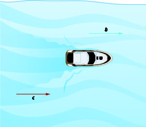
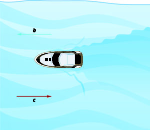
The images below show how a river current affects the speed at which a boat is actually travelling. We’ll call the speed of the boat in still water [latex]b[/latex] and the speed of the river current [latex]c[/latex].
The boat is going downstream, in the same direction as the river current. The current helps push the boat, so the boat’s actual speed is faster than its speed in still water. The actual speed at which the boat is moving is [latex]b+c[/latex].
Now, the boat is going upstream, opposite to the river current. The current is going against the boat, so the boat’s actual speed is slower than its speed in still water. The actual speed of the boat is [latex]b-c[/latex].
We’ll put some numbers to this situation in the next example.
EXAMPLE
Translate to a system of equations and then solve.
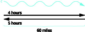
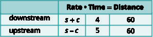
A river cruise ship sailed 60 miles downstream for 4 hours and then took 5 hours sailing upstream to return to the dock. Find the speed of the ship in still water and the speed of the river current.
In the next video, we present another example of a uniform motion problem which can be solved with a system of linear equations.
Candela Citations
- Revision and Adaptation. Provided by: Lumen Learning. License: CC BY: Attribution
- College Algebra. Authored by: Abramson, Jay et al.. Provided by: OpenStax. Located at: http://cnx.org/contents/9b08c294-057f-4201-9f48-5d6ad992740d@5.2. License: CC BY: Attribution. License Terms: Download for free at http://cnx.org/contents/9b08c294-057f-4201-9f48-5d6ad992740d@5.2
- Solving Systems of Equations using Elimination. Authored by: James Sousa (Mathispower4u.com). Located at: https://youtu.be/ova8GSmPV4o. License: CC BY: Attribution
- Question ID 115164, 115120, 115110. Authored by: Shabazian, Roy. License: CC BY: Attribution. License Terms: IMathAS Community License CC-BY + GPL
- Beginning and Intermediate Algebra. Authored by: Wallace, Tyler. Located at: http://www.wallace.ccfaculty.org/book/book.html. License: CC BY: Attribution
- Question ID 29699. Authored by: McClure, Caren. License: CC BY: Attribution. License Terms: IMathAS Community License CC-BY + GPL
- Question ID 23774. Authored by: Roy Shahbazian. License: CC BY: Attribution. License Terms: IMathAS Community License CC-BY + GPL
- Question ID 8589. Authored by: Greg Harbaugh. License: CC BY: Attribution. License Terms: IMathAS Community License CC-BY + GPL
- Question ID 2239. Authored by: Morales, Lawrence. License: CC BY: Attribution. License Terms: IMathAS Community License CC-BY + GPL
- Ex: System of Equations Application - Mixture Problem.. Authored by: James Sousa (Mathispower4u.com) for Lumen Learning.. Located at: https://youtu.be/4s5MCqphpKo.. License: CC BY: Attribution
- Beginning and Intermediate Algebra Textbook. . Authored by: Tyler Wallace. Located at: http://www.wallace.ccfaculty.org/book/book.html.%20. License: CC BY: Attribution
- Ex: System of Equations Application - Plane and Wind problem. Authored by: James Sousa (Mathispower4u.com). Located at: https://www.youtube.com/watch?v=OuxMYTqDhxw. License: CC BY: Attribution
- Intermediate Algebra . Authored by: Lynn Marecek et al.. Provided by: OpenStax. Located at: http://cnx.org/contents/02776133-d49d-49cb-bfaa-67c7f61b25a1@4.13. License: CC BY: Attribution. License Terms: Download for free at http://cnx.org/contents/02776133-d49d-49cb-bfaa-67c7f61b25a1@4.13
- Precalculus. Authored by: OpenStax College. Provided by: OpenStax. Located at: http://cnx.org/contents/fd53eae1-fa23-47c7-bb1b-972349835c3c@5.175:1/Preface. License: CC BY: Attribution
- Rates retrieved Aug 2, 2010 from http://www.budgettruck.com and http://www.uhaul.com/ ↵