At the start of this module, you were wondering whether you could earn a profit by making bikes and were given a profit function.
[latex]P\left(x\right)=R\left(x\right)-C\left(x\right)[/latex]
where
[latex]x[/latex] = the number of bikes produced and sold
[latex]P(x)[/latex] = profit as a function of x
[latex]R(x)[/latex] = revenue as a function of x
[latex]C(x)[/latex] = cost as a function of x
Profit, revenue, and cost are all linear functions. They are a function of the number of bikes sold. Remember that you were planning to sell each bike for $600 and it cost you $1,600 for fixed costs plus $200 per bike.
Since you take in $600 for each bike you sell, revenue is:
[latex]R\left(x\right)=600x[/latex]
Your costs are $200 per bike plus a fixed cost of $1600, so your overall cost is:
[latex]C\left(x\right)=200x+1600[/latex]
That means that profit becomes:
[latex]P\left(x\right)=600x-\left(200x+1600\right)[/latex]
[latex]=400x-1600[/latex]
With that in mind, let’s take another look at the table. The profit is found by subtracting the cost function from the revenue function for each number of bikes.
| Number of bikes ([latex]x[/latex]) | Profit ($) |
| 2 | [latex]400\left(2\right)-1600=-800[/latex] (loss) |
| 5 | [latex]400\left(5\right)-1600=400[/latex] |
| 10 | [latex]400\left(10\right)-1600=2400[/latex] |
That still doesn’t explain how to figure out the break-even point, the number of bikes for which the revenue equals the costs.
One way is to set the functions equal to one another and solve for [latex]x[/latex].
[latex]R\left(x\right)=C\left(x\right)[/latex]
[latex]600x=200x+1600[/latex]
[latex]400x=1600[/latex]
[latex]x=4[/latex]
That means that if you sell 4 bikes, you will take in the same amount you spent to make the bikes. So selling less than 4 bikes will result in a loss and selling more than 4 bikes will result in a profit.
Another method for finding the break-even point is by graphing the two functions. You can use whichever method of graphing you find useful.
To plot points, for example, make a list of values for each function. Then use them to determine coordinates that you can plot.
[latex]R\left(x\right)=600x[/latex]
| [latex]x[/latex] | [latex]R(x)[/latex] | [latex](x, R(x))[/latex] |
| 0 | 0 | (0, 0) |
| 2 | 1200 | (2, 1200) |
| 4 | 2400 | (4, 2400) |
| 6 | 3600 | (6, 3600) |
| 8 | 4800 | (8, 4800) |
[latex]C\left(x\right)=200x+1600[/latex]
| [latex]x[/latex] | [latex]C(x)[/latex] | [latex](x, C(x))[/latex] |
| 0 | 1600 | (0, 1600) |
| 2 | 2000 | (2, 2000) |
| 4 | 2400 | (4, 2400) |
| 6 | 2800 | (6, 2800) |
| 8 | 3200 | (8, 3200) |
To use the slope and y-intercept method, first find the y-intercept by setting x = 0. Then determine the slope as the coefficient of the variable, which is the m value.
| [latex]R(x)[/latex] | [latex]C(x)[/latex] |
| y-intercept = 0 | y-intercept = 1600 |
| slope = 600 | slope = 200 |
Using this information, the functions can be graphed
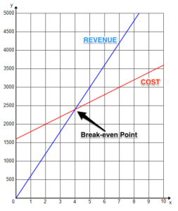
Now we can see the break-even point right away. It is the point at which the cost function intersects the revenue function. It occurs when [latex]x=4[/latex]. At this point you neither make a profit nor incur a loss.
The last question to consider is how changing your price affects your profit. If your costs remain the same, increasing the price you charge will shift your break-even point to a lower number of bikes and increase your revenue for every value of [latex]x[/latex]. However, people may not buy as many bikes. Lowering your price will shift your break-even point to a higher number of bikes and decrease your revenue for every value of [latex]x[/latex]. However, more people may buy your bikes.
Let’s take a look at the graphs for two other possible prices.
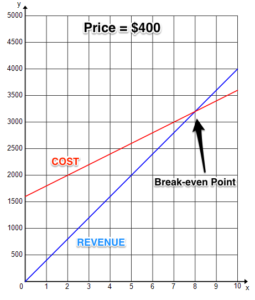
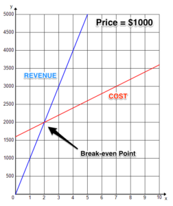
Graphing lets you quickly see a visual representation of the functions and how they are related to one another. Notice how the break-even point shifts to 8 bikes for a lower price and only 2 bikes for a higher price.
So writing, graphing, and comparing linear functions can be quite useful. As for deciding what price people are willing to pay for your bike, that’s a whole different topic!
Candela Citations
- Putting It Together: Linear and Absolute Value Functions. Authored by: Lumen Learning. License: CC BY: Attribution