Learning Goals
After completing this section, you should feel comfortable performing these skills.
- Interpret the median of a data set.
- Interpret the mean of a data set.
- Identify whether a data set is left-skewed, symmetric, or right-skewed.
- Identify in which data set the mean is greater than, less than, or approximately equal to the median.
- Identify which of the mean or median is resistant to skew.
Click on a skill above to jump to its location in this section.
When examining the distribution of a quantitative variable using a histogram or a dotplot, we often find that the distribution follows a bell shape with a mound of observances in the middle of the distribution and even amounts of data falling to the right and left. But sometimes a distribution’s values are bunched up to one side or the other, with a few observations stretching way out to the other side. You may recall from What to Know About Applications of Histograms: 3D that there are specialized statistical terms we use for these different distribution shapes: skewness and symmetry. In this section, you’ll learn that there are certain ways the mean of the data relates to the median under these different shapes.
Skewness
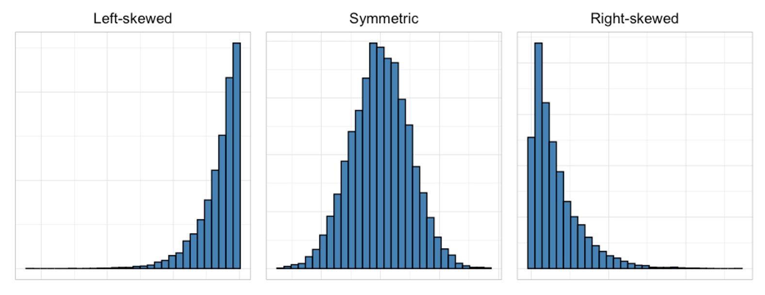
Recall that we say a quantitative variable has a right-skewed distribution or a positive skew if there is a “tail” of infrequent values on the right (upper) end of the distribution. We say a data set has an approximately symmetric distribution if values are similarly distributed on either side of the mean/median. We say a data set has a left-skewed distribution or a negative skew if there is a “tail” of infrequent values on the left (lower) end of the distribution.
skewed distributions
I’d like an animation here (super simple) of a data set that moves from right skew to symmetry to left skew with a slider students can manipulate. The labels would change over the slider: right skew / roughly symmetric / roughly symmetric / left skew.
Refresh your memory for how to describe the shape of a histogram by trying the question in the interactive example below.
interactive example
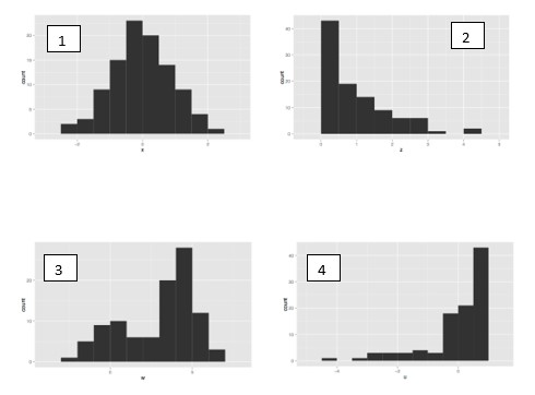
Several histograms are displayed below. Provide a description of the shape of each.
In the next activity, you’ll need to calculate and interpret the mean and median in skewed distributions. Let’s get some practice with these skills using data collected around the T.V. show Friends.
Mean and Median
Friends was a popular American television show that aired from 1994 to 2004. The show followed a group of six friends living in New York City and chronicled their relationships and day-to-day adventures. The show became known in popular culture for its comedy and for the closeness of its cast.[1]
The following table lists the number of U.S. viewers of each episode of the [latex]10[/latex]th and final season of Friends.[2]
| Episode Number | Episode Title | Air Date | U.S. Viewers (Millions) |
| 1 | The One After Joey and Rachel Kiss | 9/25/03 | [latex]24.54[/latex] |
| 2 | The One Where Ross Is Fine | 10/2/03 | [latex]22.38[/latex] |
| 3 | The One with Ross’s Tan | 10/9/03 | [latex]21.87[/latex] |
| 4 | The One with the Cake | 10/23/03 | [latex]18.77[/latex] |
| 5 | The One Where Rachel’s Sister Babysits | 10/30/03 | [latex]19.37[/latex] |
| 6 | The One with Ross’s Grant | 11/6/03 | [latex]20.38[/latex] |
| 7 | The One with the Home Study | 11/13/03 | [latex]20.21[/latex] |
| 8 | The One with the Late Thanksgiving | 11/20/03 | [latex]20.66[/latex] |
| 9 | The One with the Birth Mother | 1/8/04 | [latex]25.49[/latex] |
| 10 | The One Where Chandler Gets Caught | 1/15/04 | [latex]26.68[/latex] |
| 11 | The One Where the Stripper Cries | 2/5/04 | [latex]24.91[/latex] |
| 12 | The One with Phoebe’s Wedding | 2/12/04 | [latex]25.9[/latex] |
| 13 | The One Where Joey Speaks French | 2/19/04 | [latex]24.27[/latex] |
| 14 | The One with Princess Consuela | 2/26/04 | [latex]22.83[/latex] |
| 15 | The One Where Estelle Dies | 4/22/04 | [latex]22.64[/latex] |
| 16 | The One with Rachel’s Going Away Party | 4/29/04 | [latex]24.51[/latex] |
| 17 | The Last One* | 5/6/04 | [latex]52.46[/latex] |
| 18 | The Last One* | 5/6/04 | [latex]52.46[/latex] |
We’ll use technology to analyze this data set.
Go to the Describing and Exploring Quantitative Variables tool at https://dcmathpathways.shinyapps.io/EDA_quantitative/.
Step 1) Select the Single Group tab.
Step 2) Locate the drop-down menu under Enter Data and select Your Own.
Step 3) Under Do you have, select Individual Observations.
Step 4) Under Name of Variable, type “U.S. Viewers (Millions).”
Step 5) Cut and paste or enter the data presented in the above table for U.S. Viewers (Millions).
interactive example
In the following questions, you’ll need to interpret the mean and median of the data set. Recall that we think of the mean as the “average” data value and the median as the 50th percentile, the value that splits the data in half. If needed, you may return to Calculating the Mean and Median of a Data Set: What to Know for a refresher of these interpretations of mean and median.
Example: Let’s say the mean of a data set is given as 10.5 and the median as 11. Which of the following statements are true? Explain.
- The median tells us a typical value for this data set. That is, if we took all the values and spread them evenly about, each value would be about 11.
- About half the data values fall below 11 and half fall above.
- The most common data value appearing is 10.5.
- A typical data value for this set is 10.5. That is, if we distributed the sum of all the values evenly, each value would be about 10.5.
Now it’s your turn to use the data set for the TV show Friends to answer the questions below.
question 1
question 2
question 3
question 4
question 5
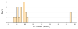
For this question, use the following histogram of the Season 10 Friends viewership data.
question 6
question 7
question 8
question 9
Mean and Median Under Skew
effects of skew on mean and median
[Perspective video — a 3-instructor video that shows how to think about the tail and the two outliers in the data above together with the fact that the mean is larger than the median to begin to understand that the mean tends to be pulled to the right of the median under a right skew.]
For each of the plots of data below, choose the description that matches the shape of the data’s distribution, and then select the choice that gives the relationship between the mean and median for those data. Base your answers on the understanding you established in Questions 1 – 9 about the direction the mean was pulled in under the skewness in the data set.
question 10
question 11
question 12
Resistance
Resistant and Nonresistant Measures of Center
[Worked example – a 3-instructor video showing a symmetric data set with the mean and median identical, then, skewing the distribution to show what happens to the mean while the median remains in place.]
question 13
Hopefully, you have noticed that when a distribution is symmetric, the mean and median occupy the same value. But under a skew, the mean is “pulled” in the direction of the outliers: greater than the median in the case of positive (right) skew, and less than the median in the case of negative (left) skew. It appears that the mean is affected by the presence of outliers while the median is not.
Looking ahead
Broadly speaking, we consider a value in a data set to be an outlier if that value is unusual or extreme, given the other values in the data set.
Suppose you have two groups of people:
- Group 1 is made up of five professional basketball players, and Group 2 is made up of four professional basketball players and one kindergartener.
- Dataset 1 contains the number of three-pointers each person in Group 1 can make in one minute. Dataset 2 contains the number of three-pointers each person in Group 2 can make in an hour.
question 14
Summary
In this section, you’ve learned about skewed distributions vs. symmetric distributions and how skew affects the mean of a data distribution. You also got some practice calculating and interpreting the mean and median of a data set. Let’s summarize where these skills showed up in the material.
- In Question 1, you calculated the median of a data set, and interpreted the median in Question 2.
- In Question 3, you calculated the mean of a data set, and interpreted the mean in Question 4.
- In Question 5, you began to see how the mean and median relate in a distribution.
- In Questions 6, and 10 – 13, you used statistical terms for skew and extreme values to describe the features of a data set, and began to make connections between the mean and median under differently shaped distributions.
- In Questions 7 -9, you interpreted the mean and median to make connections between them and the data distribution.
- In Question 13, you identified which of the mean or median is resistant to skew.
Being able to interpret the mean and median with regard to the shape of a distribution and the presence of outliers will be essential skills to use when assessing claims made about data that rely on measures of center. If you feel comfortable with these skills, please move on to the activity!
- Encyclopedia Britannica. (n.d.). Friends. In Encyclopedia Britannica.com. https://www.britannica.com/topic/Friends ↵
- Mock, T. (2020). A weekly data project aimed at the R ecosystem. TidyTuesday. https://github.com/rfordatascience/tidytuesday/blob/master/data/2020/2020-09-08/readme.md#friends_infocsv ↵